Digital Image Processing Algorithms Research Based on FPGA

Transcription

1 Digital Image Processing Algorithms Research Based on FPGA By Haifeng Xu Supervisor: Prof. Wenqing Zhao & Senior Engineer Gengsheng Chen Examiner: Prof. Lirong, Zheng Thesis Period: Aug 2009 Mar 2010 Department of Microelectronics, School of Information Science and Technology Fudan University, Shanghai, China Royoal Institute of Technology (KTH), Stockholm, Sweden

2 Acknowledgement I am deeply indebted to a large number of people who have helped me in my graduate school. My deepest gratitude goes first and foremost to Prof. Wenqing Zhao, Senior Engineer Gengsheng Chen, Prof. Lirong Zheng, Prof. Shili Zhang, Prof. Ran Liu for their constant encouragement and guidance. They have walked me through all the stages of the writing of this thesis and given me a lot of help during research. Without their consistent and illuminating instruction, this thesis could not have reached its present form. I will also thank Professor Jinmei Lai, who has enrolled me as a member of CAD team at the very beginning and led me to the world of FPGA design. I am very grateful for her help. Second, I am thankful to all the teachers in Fudan University, Royal Institute of Technology, Rugao Senior School of Jiangsu Province and Jiang an Junior school of Rugao, who had taught me patiently in class, gave me wisdom, strong my competence in fundamental and essential academic. I will never forget their help, which has got me through the tough times. Third, my gratitude goes to the my seniors, Jun Chen, Liguang Chen, Wenbo Yin, Yabin Wang, Jian Wang, Haizhou Lu and Fan Yang and so on. I am very grateful for their assistance and guidance during my research. I also owe my sincere gratitude to my friends and my fellow classmates who gave me their help and time in listening to me and helping me work out my problems. I am grateful for all the cheerful chatting and laughing that they bring to my life. Shujiang Cai, Changming Pi, Wen Jiang, Hao Wu, Haixiang Bu, Fanjiong Zhang, Shaoteng Liu, Sha Liu, Shaochi Liang, Chong Shen, and Genglong Chen.etc are all warmhearted guys. I am such a lucky person to be a friend of them. Last, my thanks would go to my beloved family, my parents and grandparents, for their loving considerations and great confidence in me all through these years. i

3 Contents Acknowledgement... i Contents...ii Abstract... iv Part-I Introduction Digital TV sets Digital Video Fundamentals Broadcast Video standard Character Of Video Streams Frame Rate Video Resolution Color Space Interlacing De-interlacing Algorithms Non-motion Compensated Algorithms Linear Methods Motion Adaptive Edge-Dependent Interpolation(EDI) Motion Compensated Algorithms Goal of Thesis Structure of the Thesis Part-II Motion Estimation Motion Estimation Fundamental Block Matching Criteria Mean Absolute Deviation & Sum of Absolute Deviation Mean Squared Error Normalized Cross-Correlation Motion Estimation Algorithms Full Search (FS) Algorithm Three Step Search (TSS) Algorithm New Three Step Search (NTSS) Algorithm Four Step Search (FSS) Algorithm Diamond Search (DS) Algorithm Cross Search (CS) Algorithm Cross-Diamond Search (CDS) Algorithm Block-Based Gradient Descent Algorithm Algorithm Comparison Part-III Down-Sampled Three Step Search Algorithm Motion Vector Distribution Characteristic Down Sampled Three Step Search Algorithm Algorithm Simulation ii

4 3.1 Power Signal-to-Noise Ratio(PSNR) comparison Mean Square Error(MSE) and Mean Absolute Deviation (MAD) Comparison Algorithm Complexity Comparison Visual Effect Comparison Part IV Motion Estimation in De-interlace Motion Compensated Linear Method Weaver algorithm Motion Compensated Weaver algorithm using DSDTSS Motion Compensated Weaver using NTSS System Framework Receiver Module Clock Generator module Format Generator Module Flow Control Module Transmitter Module Synthesis Result References iii

5 Abstract As we can find through the development of TV systems in America, the digital TV related digital broadcasting is just the road we would walk into. Nowadays digital television is prevailing in China, and the government is promoting the popularity of digital television. However, because of the economic development, analog television will still take its place in the TV market during a long period. But the broadcasting system has not been reformed, as a result, we should not only take use of the traditional analog system we already have, but also improve the quality of the pictures of analog system. With the high-speed development of high-end television, the research and application of digital television technique, the flaws caused by interlaced scan in traditional analog television, such as color-crawling, flicker and fast-moved object's boundary blur and zigzag, are more and more obvious. Therefore the conversion of interlaced scan to progressing scan, which is de-interlacing, is an important part of current television production. At present there are many kinds of TV sets appearing in the market. They are based on digital processing technology and use various digital methods to process the interlaced, low-field rate video data, including the de-interlacing and field rate conversion. The digital process chip of television is the heart of the new-fashioned TV set, and is the reason of visual quality improvement. As a requirement of real time television signal processing, most of these chips has developed novel hardware architecture or data processing algorithm. So far, the most quality effective algorithm is based on motion compensation, in which motion detection and motion estimation will be inevitably involved, in despite of the high computation cost. in video processing chips, the performance and complexity of motion estimation algorithm have a direct impact on speed area and power consumption of chips. Also, motion estimation determined the efficiency of the coding algorithms in video compression. This thesis proposes a Down-sampled Diamond NTSS algorithm (DSD-NTSS) based on New Three Step Search (NTSS) algorithm, taking both performance and complexity of motion estimation algorithms into consideration. The proposed DSD-NTSS algorithm makes use of the similarity of neighboring pixels in the same image and down-samples pixels in the reference blocks with the decussate pattern to iv

6 reduce the computation cost. Experiment results show that DSD-NTSS is a better tradeoff in the terms of performance and complexity. The proposed DSD-NTSS reduces the computation cost by half compared with NTSS when having the equivalent image quality. Further compared with Four Step Search(FSS) Diamond Search(DS) Three Step Search(TSS) and some other fast searching algorithms, the proposed DSD-NTSS generally surpasses in performance and complexity. This thesis focuses on a novel computation-release motion estimation algorithm in video post-processing system and researches the FPGA design of the system. Key words: video post-processing, motion estimation, motion detection, de-interlace, Field Programmable Gate Array (FPGA). v

7 Part-I Introduction 1 Digital TV sets As consumers, we find many video systems in our daily lives. However, from the embedded developer s viewpoint, video represents a tangled web of different resolutions, formats, standards, sources and displays [1]. Later, all these characters of video systems will be explained in detail. We can divide the TV signal into two categories: First, analog TV signal. Before the mid-1990 s, nearly all video was in analog form. It has developed through decades, and the related technology has reached its peak.in the United States, analog TV signal broadcasting system should be replaced by the next-generation technology according to the government policy. Despite the fact that the analog TV signal is old fashioned, most of the developing countries are using this kind of broadcasting system, and all the TV sets sold today support this signal. Second, digital TV signal. It represents the next-generation TV broadcasting technology. As the new technology, the digital TV system will overcome the flaws of analog TV signal, such as color-crawling, flicker and fast-moving object's boundary blur and zigzag. But the new technology usually will cost heftily, and the whole broadcast system replacement needs tremendous investments. Before there comes any profitable business model, digital TV broadcast will be just a dream. Especially in developing countries, the analog TV broadcasting system will stand for a long time E E E E E+07 Number Of DTV User E Fig 1: Development of Digital TV in China In China, digital TV is prevailing almost all over the country. We can find this trend from the figure above. We are now at the transition period, during which the 1

8 two kinds of TV signal will be coexisting. There are millions of families in China that will finally pay the bill for the digital TV sets. This is a great opportunity for TV set manufacturers that in turn also want to find a path into this gigantic market. The most popular way is to use advanced digital processing method to enhance the image visual effect during this special period. A digital TV set makes use of an ASIC chip as its brain. This chip integrates most of the video processing functions, such as de-interlacing, format conversion, de-noising, scaling and so on. With this chip, the digital TV set will give us a brand new visual perception feeling. The digital TV set is a perfect choice for the Chinese consumers pursuing better visual quality during the phase of TV broadcasting system renovation. 2 Digital Video Fundamentals Digital video comprises of a series of orthogonal bitmap digital images displayed in rapid succession at a constant rate. And these digital images are called frames when referred to in the field of video processing. [2, 3] Digital video was first introduced commercially in 1986 with the Sony D-1 format, which has changed the video recording methodology from the high-band analog form to digital form. But because of the large expense, D-1 format was used primary by large television networks, instead of salaried person. It was doomed to be replaced by other cheaper systems. Later, consumer digital video appeared in the form of QuickTime, which is the Apple Computer s multimedia framework for time based and streaming data format. While low-quality at first, consumer digital video increased rapidly in quality with the introduction of playback standards such as MPEG-1 and MPEG-2, further, the introduction of the DV tape format. The widespread adoption of digital video has drastically reduced the bandwidth compared with its analog counterpart. And the popularity of digital video also sent consumers its advantages, including better signal to noise performance, improved bandwidth utilization and reduction in storage space through digital compression techniques. Since the crude signal we collect is in analog form, there comes the question how could digital video be obtained. The answer is video digitizing, which is the method we turn to. At its root, digitizing video involves both sampling and quantizing the 2

9 analog video signal. Sampling entails dividing the frame into pixels and assigning relative amplitude values based on the intensities of color space components in each pixel. Quantization is the process that determines these discrete amplitude values assigned during the sampling process. However, the round-off error is the main problem caused by quantization. The good news is that the round-off error can be eliminated by increasing the number of bits per pixel, because the human visual system could not distinguish from the difference of one. Nowadays, 8 bit video is common in consumer applications, where a value of 0 is black and 255 is white, for each color channel. 2.1 Broadcast Video standard Video standards differ in the way they encode brightness and color information. Two standards dominate the broadcast television realm NTSC and PAL. The distribution of video standards is shown in fig.2. NTSC, devised by the National Television System Committee, is prevalent in Asia and Northern America, whereas PAL ( Phase Alternation Line ) dominates Europe and Southern America. PAL was developed as an offshoot of NTSC, improving on its color distortion performance. A third standard, SECAM(Sequential Color With Memory), is popular in France and parts of Eastern Europe, but many of these areas use PAL as well. Our discussions will center on PAL systems. Fig 2: NTSC-PAL-SECAM distribution [4] 2.2 Character Of Video Streams Frame Rate We can find expressions, such as 50p, 30p and 25p, in some circumstance. The number in these expressions illustrates that, 50 for example, there are 50 digital images per second in video. Here the number of digital images per second 3

10 is called frame rate, ranges from 6 to 120 or more frames per second. The minimum frame rate to achieve the illusion of a moving image is about 15 frames per second. Table 1 illustrates the frame rate of the video standards mentioned above. There are other expressions, such as 50i and 60i, which are different from those mentioned before. Since they refer to another concept introduced later, then their meaning will be made clear. Table 1: Frame rate of PAL,SECAM and NTSC standards Broadcasting Video Standard Frame Rate(frames/s) PAL 25 SECAM NTSC Video Resolution As mentioned before, the sampling entails dividing the frame into small regions, called pixels. Here the size of these small regions dominants video resolution. While going further, video resolution can be decomposed into two items, horizontal resolution and vertical resolutions. Horizontal resolution indicates the number of pixels on each line of the image, while vertical resolution designates how many horizontal lines are displayed on the screen to create the entire frame. Consequently, video resolution can be put in the way of multiplication of horizontal resolution and vertical resolution. In the digital domain standard-definition television (SDTV) is specified as for NTSC and for PAL or SECAM resolution. High definition systems (HD) often employ progressive scanning and can have much higher horizontal and vertical resolutions than SD systems. In this thesis, we will focus on SD systems rather than HD systems, but most of our discussion also generalizes to the HD systems Color Space There are many different ways of representing color, such as YCbCr and RGB, and each color system is suited for different purposes. The most fundamental representation is RGB color space. RGB stands for Red Green Blue, and it is a color system commonly employed in computer graphics displays. As the three primary colors that sum to form white, they can 4

11 combine in proportion to create almost any color in the visible spectrum. One of the disadvantages of the RGB color system is that each of the three channels is highly correlated with the other two, which could be poorly compressed. There is another commonly used color system, YCbCr, employed less correlation among channels to reduce required transmission bandwidths and increase video compression ratios. The YCbCr color system separates a luminance component from two chrominance components through the equations below: Y R G B; Cb R G B 128; Cr R G B 128; Interlacing Digital video cameras come in two different image capture methods: interlaced and progressive scan. From fig.3 we can find the difference between their productions. Interlacing was invented as a way to achieve good visual quality within the limitations of a narrow bandwidth. Interlaced cameras record the horizontal lines frame by frame in such a pattern: odd-numbered lines are first scanned, followed by the even-numbered lines are scanned, and then the odd-numbered lines are scanned again, and so on. In an interlaced video, a frame consists of two halves of an image. Those halves are referred to individually as fields. Two consecutive fields compose a full frame. If an interlaced video has a frame rate of 25 frames per second, the field rate is 30 fields per second. Abbreviated video resolution specifications often include an i to indicate interlacing. Up to now, we can look back to the unresolved problem in Fig 3: Progressive Vs Interlaced Scan Because each frame of an interlaced video is composed of two fields that are 5

12 captured at different moments, the interlaced video will suffer from motion artifacts if the recorded objects are moving fast enough to be in different positions. And the panel TV sets are progressive scan systems, so the interlaced video will inevitably cause visual artifacts. In order to deal with these artifacts, a process known as de-interlacing can be used for converting an interlaced stream to be processed by progressive scan devices, such as TFT TV-sets, projectors, and plasma panels. De-interlacing systems are integrated in to progressive scan television displays in order to provide the best possible picture quality for interlaced video. This de-interlacing system is the primary topic of this thesis. 3 De-interlacing Algorithms De-interlacing, which is a process generating progressive video from interlaced video, has been widely used to reduce the visual effects of artifacts caused by interlaced video. Moreover, HDTV systems support the progressive scan to improve the visual quality. However, the interlaced scan may still be employed in view of compatibility with existing TV and camera systems. Thus, the multi-format digital broadcast and progressive display require the de-interlacing technology [4-6]. The de-interlacing task is illustrated in Fig.4. The input consecutive fields, containing samples of either the odd or the even lines of an image, have to be converted to frames. These frames represent the same image as the corresponding input fields but contain the omitted lines. We can give this process a mathematical expression, let the output frame be F o ( x, n). F( x, n)( y mod 2 n mod 2) Fo ( x, n) Fi ( x, n)( otherwise ) In the equation above, ( x, n) indicates the interpolated pixels. F i n-1 n-1 n n Fig 4: The De-interlacing Task 6

13 The algorithms of de-interlacing could be divided into two categories: non-motion compensated and motion compensated. The most advanced de-interlacing algorithms use motion compensation. It is only since the mid-1990 s that motion estimators have been feasible at a consumer price level. In this thesis, the main focus is motion compensated algorithm because of its better visual effects. 3.1 Non-motion Compensated Algorithms Linear Methods Generally, linear methods can be described by (1), shown below, with 0 g( k, m) the impulse response of the filter in the VT domain and u y. 1 Similar to 0 u y, we also defineu x. The actual choice of g ( k, m) determines 1 whether it is a spatial, temporal, or spatio-temporal filter. F( x, n),( y mod 2 n mod 2) F( x, n) F( x kuy, n m) g( k, m),( k m) mod 2 1..(1) k ( k, m) {..., 1,0,1,...},( otherwise ) In linear methods, the missing pixels are obtained by linear interpolation of known pixels in temporal and/or spatial directions. The linear techniques are based on the assumption that the video is continuous in both temporal and spatial directions. The interpolation along temporal direction is called temporal filtering, while the one along spatial direction is termed spatial filtering. Pure temporal filtering implies a spatial all pass. Consequently, there is no degradation of stationary images. Similarly, the pure spatial filtering provides all-pass characteristic in the temporal frequency domain. The pure spatial filtering is mostly applied to tackle moving images. A temporal-spatial filter would theoretically solve the de-interlacing problem if the signal were bandwidth limited prior to interlacing. Specially, Bob is the most popular spatial de-interlacing technique for which g ( k,0) 0. 5 for k 1, 1, and h ( k, m) 0. While the most famous temporal de-interlacing method, Weave, results from selecting h ( 0, 1) 1, and 7

14 h ( k, m) 0 otherwise Motion Adaptive Besides the continuation property employed in linear techniques, more information can be derived from the video to enhance the de-interlacing effect. All motion adaptive methods are defined by (2) below. In the motion-adaptive methods, the motion possibilities of the missing pixels are got from the video. With the motion possibilities of the missing pixels, the de-interlacing effect can be greatly enhanced. The motion possibility is applied to switch or preferably fade between two processing modes, one optimal for stationary and the other for moving image parts [7]. F( x, n),( y mod 2 n mod 2) Fo ( x, n) (2) F st( x, n) (1 ) Fmot ( x, n)( otherwise ) where F st ( x, n) is the value obtained by the method optimal for stationary image while F mot ( x, n) for moving image. The main problem of motion-adaptive methods is the robustness of motion detection. The de-interlaced image will greatly be degenerated if motion detection is wrong Edge-Dependent Interpolation(EDI) Contrary to motion-adaptive methods that use the temporal correlation of the video to improve the e-interlacing effect, in EDI methods, the correlations in spatial direction are taken into account. The EDI methods are based on the assumption that the missing pixels tend to be the same as the pixels along the lines the missing pixels belong to. According to the spatial correlations, the edge direction can be detected. Denote (d,1) as the edge direction of one missing pixel F ( x, y, n), the F ( x, y, n) obtained by EDI methods can be described by (3) as follows [8]. F( x d, y 1, n) F( x d, y 1, n) F( x, y, n) (3) 2 EDI methods preserve the edges of the images, thus preserve the resolution of the image. Furthermore, the EDI methods actually are spatial filtering 8

15 methods. The correctness of edge direction is the key parameter for detail preserving result. 3.2 Motion Compensated Algorithms Similar to many other algorithms, motion compensated methods try to interpolate in the direction with the highest correlation. With motion vectors available, this is an interpolation along the motion trajectory. Motion compensation allows us to virtually convert a moving sequence into a stationary one. Methods that perform better for stationary than for moving image parts will profit from motion compensation. Replacing the pixels F ( x, y, n) with F( x p, y q, n m) converts a non-mc method to an MC version, the motion vector is md ( p, q, m). Indeed, MC field-insertion, MC field-averaging, MC VT (Vertical-Temporal) filtering, MC adaptive filtering, and combinations with edge adaption have been proposed by many video researchers. the nth field the (n+1)th field Motion Estimation motion vector Motion Compensation the nth field Fig 5: Motion Compensation Illustration 4 Goal of Thesis The main issues involved in motion compensation methods are motion estimation and the reliability of motion vectors. If the calculated motion vector is wrong, the compensated image will be severely corrupted. Since the motion vector can be wrong, the robustness of motion vector becomes a key problem in motion compensation algorithm. Also the computational cost of such algorithm is high since it uses the motion estimation, in which the block matching method is adopted [9]. In this thesis we will focus on the algorithm to reduce the computation cost. 9

16 5 Structure of the Thesis In the current chapter, the background of de-interlacing and related algorithms has been briefly introduced. The second chapter is devoted to the realization of the motion estimation algorithms. The third chapter presents a newly proposed algorithm based on the research for this thesis. The fourth chapter concerns the implementation of this specific algorithm into de-interlace system. 10

17 Part-II Motion Estimation Motion estimation, for a long time, used to be a specialized research area that had not much to do with general image processing. This separation had two reasons. First, the techniques used to analyze motion in image sequences are quite different. Second, the extensive amount of storage space and computing power required made image sequence analysis available only to a few specialized institutions that could afford the expensive specialized equipment. With the development of semiconductor industry, both reasons are no longer true. Because of the general progress in image processing, the more advanced methods used in motion analysis no longer differ from those used for other image processing tasks. The rapid progress in computer hardware and algorithms makes the analysis of image sequences now feasible even on standard personal computers and workstations [9]. Motion is indeed a powerful feature of video sequence. We may compare the integration of motion analysis into mainstream image processing with the transition from still photography to motion pictures. Only image sequence analysis allows us to recognize and analyze dynamic processes. Thus far-reaching capabilities become available for scientific and engineering applications including the study of flow; transport; biological growth processes from the molecular to the ecosystem level; industrial processes; traffic autonomous vehicles and robots to name just a few application areas. In short, everything that causes temporal changes or makes them visible in our world is a potential subject for image sequence analysis. In a continuous video sequence, there is a lot of relevance between the adjacent frames. For motion image the most situation is that only very few part of images in motion, the content difference between two neighboring video frame in same identical scene is not obvious, or that the content of the latter and the preceding have many overlap parts, that is to say that the two frame have strong time relativity. The goal of motion estimation is to find the relevance between frames and the product of motion estimation is motion vector of pixels or blocks, which will be taken use of by other algorithms to finish their mission. As described in part I, motion estimation and motion compensation are used in some de-interlacing algorithms. Also motion estimation plays an important role in other areas, such as video compression, computer vision and de-noising [10]. The 11

18 accuracy requirement of different fields varies. For example, computer vision and military tracking need the motion vector to show the actual movement; at the same time, video compression cares more about the compression ratio rather than motion vector accuracy. The visual quality of motion compensated de-interlacing algorithms lean upon the accuracy of motion vectors. 1 Motion Estimation Fundamental We will think about changes spontaneously, when motion is mentioned. Thus we start with analysis of the differences between two images of a sequence. Figure 6 shows two continuous images from a landscape sequence. There are difference between the upper and bottom which is not that obvious from direct comparison. But if we subtract one image from another, the difference comes into our visibility immediately, which is illustrated in Figure 7. (a) (b) Figure 6: Two consecutive images from a landscape scene At the top middle, a petal is moving upward, and another petal also appears on the scene at the lower left. If we observe the image edges, we notice that the images have shifted slightly in a horizontal direction. The background movement could be discovered through the subtraction image, which may be caused by the position change of the camera. In the difference image Figure 7, all the edges of the objects appear as bright lines. However, the image is dark where the spatial gray value changes are small. Consequently, we can detect motion only in the parts of an image that show gray value changes. This simple observation points out the central role of spatial gray value changes for motion determination. We can get a conclusion that motion can cause temporal gray value changes in image. But unfortunately the reverse statement that all temporal gray value changes are due to motion is not correct. 12

19 Because gay value change can also be caused by illumination change like day and night, we can observe this kind of phenomenon in our daily life. Figure 7: Difference between images It is obvious that motion analysis helps us considerably in understanding such a scene. It would be much harder to detect moving background. There are several realization of motion estimation, such as pixel-based motion estimation, block-based motion estimation and grid-based motion estimation. In this thesis the realization of block-based motion estimation is our focus, since its popularity and better performance. The basic idea of block-based motion estimation (as shown in Figure 8) is to divide each frame of image sequence into many non-overlapping macro blocks, and that all the block-pixel displacement are the same, then for each block in current frame find the most similar block namely matching block in given scope to the front or after frame(reference frame) according to certain matching criteria, and figure out motion displacement from the relative position of the matching and current block and the motion displacement is the motion vector of current block. Current Frame CMP Motion Vector Reference Frame Figure 8: Idea of Block-Based Motion Estimation 13

20 Obviously the main objective of motion estimation for de-interlace is to make the motion vector as accuracy as possible. Because the block-matching needs pixel comparison between the before and after frame, so if full search algorithm (that is compare with all possible points in exhaustive reference frame region and then find the overall merits) is used, the computation is very large. In order to be further implemented into hardware, the motion estimation should also take computation cost into consideration. Also the de-interlaced video has half image information, so we should first convert the de-interlaced image into a full image by using BOB algorithm, which will be discussed in detail later. 2 Block Matching Criteria In block-based motion estimation algorithms, each block from the current frame is matched into a block in the destination frame by shifting the current block over a predefined neighborhood of pixels in the destination frame (Search window), as shown in Figure 9. Generally, p and q are same; M is equal to N. At each shift, the sum of the distances between the gray values of the two blocks is computed. And often the best match block gives the smallest gray total difference. The difference calculation method becomes a key element and the accuracy of motion estimation relies on the matching criteria used in block-matching process [11]. p Current block N Search window M q Figure 9: Block Matching Process In the ideal case, two matching blocks have their corresponding pixels exactly equal. This is rarely true because moving objects change their shape in respect to the 14

21 observer's point of view, the light reflected from objects' surface also changes, and actually in the real world there is always noise. Furthermore, from semantic point view, in scenes containing motion there are occlusions among the objects, as well as disappearing of objects and appearing of new ones. Despite the problems of pixel by pixel correspondence, it is fast to compute and is used extensively for finding matching regions. There are many ways to compare the similarity between two blocks, some of the most often used matching criteria based on pixel differencing are mean absolute deviation (MAD), sum of absolute deviation(sad), mean squared error (MSE), and normalized cross-correlation(ncc). 2.1 Mean Absolute Deviation & Sum of Absolute Deviation In statistics, the absolute deviation of an element in a data set is the absolute difference between the element and a given point. And often this given point is the mean of the data set. The equation can be illustrated as below: (4); When used as the criteria for block matching algorithms, the calculation is made between two data sets, which are totally different from one data set condition. Certainly, some changes should be made in equation (4). The average function should be replaced by the gray value of its corresponding pixel, since the average of a pixel block cannot represent the details of image, such as contour. For example, in Figure 10, the left block is cut from one popular test sequence, susie, and the right one is coined according to the mean gray value of the left one. As we can see, these two blocks have the same average gray value, but totally different appearances. Figure 10: Two Blocks with Same Mean Value 15

22 In order to represent the similarity between two blocks, equation (4) should be changed into:. (5), Here we assume that the frame motion of objects is limited in the search window. Variables i and j are the coordinates of pixels in the block, while the x and y are the relative coordinates between two adjacent blocks. And the relative coordinates are within the range of the search window. In equation (5), one MAD between two blocks will take (2MN-1) arithmetic operations and one division. Actually for some kind of CPUs, since there is not embedded hardware division modules, the division will cost much more time than arithmetic operations, which will introduce an unacceptable delay. Also the embedded DSP module will occupy a large area in the CPU, which inevitably increases the power consumption. An easy way to avoid both draw backs is omitting the division, and another block matching criterion, Sum of Absolute Deviation (SAD), is derived:. (6). Because of its low computation cost, SAD is adopted by most of block matching algorithms. 2.2 Mean Squared Error The mean square error (MSE) of an estimator is one of many ways to quantify the difference between an estimator and the true value of the quantity being estimated. MSE is a risk function, corresponding to the expected value of the squared error loss or quadratic loss. MSE measures the average of the square of the "error." The error is the amount by which the estimator differs from the quantity to be estimated. The difference occurs because of randomness or because the estimator doesn't account for information that could produce a more accurate estimate. The expression of MSE is:.. (7). Instead of taking the absolute value, we squared it and get MSE. From equation (7), we can find MSE has a more precise similarity judgment between two data sets. This is a result of the squaring of each term, which effectively weights large errors more heavily than small ones. For example, 2 and 4 are only 4-2=2 apart. But, 2^2 and 4^2 are 16-4=12 apart. When two data sets have the same MAD compared with the reference data set, the data set, which gives a smaller MSE, is the more accurate estimator. 16

23 In order to function as a criteria for block matching, equation (7) should be converted into 2-D mode... (8) Although MSE performs better in similarity judgment, the computation is intensive. This is all because of the square function, which introduced multiplication operation. In most of the real-time video processing algorithms, MSE is not used as a block matching criteria, but just a standard for algorithm performance comparison. 2.3 Normalized Cross-Correlation Normalized cross correlation (NCC) has been commonly used as a metric to evaluate the degree of similarity (or dissimilarity) between two compared images. The main advantage of the normalized cross correlation over the cross correlation is that it is less sensitive to linear changes in the amplitude of illumination in the two compared images [12]. Furthermore, the NCC is confined in the range between 1 and 1. The maximum values or peaks of the computed correlation values indicate the matches between a template and sub-images in the sequence. The normalized cross correlation used for finding matches of a reference template of size in a scene image is defined as: (9) Where. (10). (11) And the variables x and y are the relative vertical and horizontal coordinates from the reference template. Of course, the computation cost is extraordinarily high as shown in equation (9). There is a strategy to reduce the computational load of the normalized cross correlation is to reduce data dimensionality by converting the 2D image into a 1D representation. But the computation cost is also much higher that MSE, not even MAD and SAD. In my research, SAD is used as the matching criteria; MSE and MAD are function as indication of algorithm performance. 17

24 3. Motion Estimation Algorithms The principal requirement of real-time motion estimation algorithms is to achieve at the same time high processing speed and a low computing time without scarifying in image quality. In effort to reduce the computational complexity of ME algorithms, a variety of methods have been devised such as such as block matching algorithm, parametric /motion model, optical flow, and pixel recursive technique. Among these methods, BMA seems to be the most popular method, due to its effectiveness and simplicity for both software and hardware implementations. BMA is also widely adopted by various coding standards such as MPEG-1, MPEG-2, MPEG-4, and H.264. It is obvious that full search algorithm is the simplest and most accurate strategy, which sometimes is also referred to as the exhaustive search of the brute force search. The full search (FS) gives the optimal solution, in term of prediction quality, by exhaustively searching over all possible blocks within the search window. However, the computational complexity of FS has motivated plenty of optimal but faster search strategies. Thus, efficient algorithms such as three step search algorithm (TSS), new three step search algorithm (NTSS), four step search algorithm (FSS), diamond search algorithm (DS), cross search algorithm (CS), cross diamond search algorithm (CDS) and block-based gradient descent search algorithm (BBGDS) have been developed to deal with this problem. All these algorithms (TSS, NTSS, FSS, DS, CS, CDS, BBGDS) lead to sub-optimal solutions because of the fact that only a local minimum is obtained because the algorithm assumes a monotone decreasing of the error when searching the minimum block difference, which is not always true. In the following part, all the fast search algorithms are described in detail. 3.1 Full Search (FS) Algorithm Full Search algorithm performs an exhaustive search over all possible points of the search window [10]. That is to say that one search with a search radius of 7 must perform the SAD operation on all the 225 points, which actually is time consuming task [13]. Start 18

25 Figure 11: Full Search Algorithm 3.2 Three Step Search (TSS) Algorithm Figure 12: Three Step Search Algorithm It contains three steps of search as it is illustrated in Figure 12. In the first step we check the nine points marked by black points, the coordinates of which are (i, j) (i, j-4) (i, j+4) (i-4, j) (i-4,j-4) (i-4, j+4) (i+4, j-4) (i+4, j) (i+4, j+4). In the second step we check eight points marked by red points surrounding the minimum found in the first step. In the third step we check eight points marked by pink points surrounding the minimum of the second step. Thus 25 points are checked in the TSS algorithm. The three-step search (TSS) algorithm has been widely used as the motion estimation technique in some low bit-rate video compression applications, owing to its simplicity and effectiveness [14]. 19

26 3.3 New Three Step Search (NTSS) Algorithm Figure 13: New Three Step Search Algorithm NTSS differs from TSS by assuming a center-biased checking point pattern in its first step and incorporating a halfway-stop technique for stationary or quasi-stationary blocks [15]. The details are given below : 1) In the first step, in addition to the original checking points used in TSS, eight extra points are added, which are the eight neighbors of the search window center, as shown in Figure 13. (As such, the checking point pattern is highly center-biased.) 2) A halfway-stop technique is used for stationary and quasi-stationary block in order to fast identify and then estimate the motions for these blocks: a) if the minimum difference point in the first step occurs at the search window center, stop the search. (This is called the first-step-stop.) If the minimum difference point in the first step is one of the eight neighbors of the window center, the search in the second step will be performed only for eight neighboring points of the minimum and then stop the search. (This is called the second-step-stop.) b) The block diagram of NTSS is shown in Figure 14. Clearly, it has retained the simplicity and regularity of TSS. It is seen that the only case where a complete three-step search needs to be executed is when the minimum difference point of the first step is neither the window center nor any of its eight neighboring points. Due to the use of this new 20

27 center-biased checking point pattern in the first step, the introduction of the first-step-stop technique seems quite reasonable. For such a case, the motion is really gentle and therefore the window center deems to represent the true motion vector. For the case where a second-step-stop happens, it is also easy to understand that (1)the motion is again small; (2) the execution of the second step makes the estimation more accurate (and thus is worthwhile); and (3) the possibility of finding the true motion after the second step is quite high (thus justifying the suitability of a second-step-stop). 1 st Step of NTSS 17 Checking Points true false false Decision #1 Decision #2 MV=(0,0) true 2 nd Step of NTSS 2 nd and 3 rd Step of NTSS 3 or 5 Checking MV MV Figure 14: Block Diagram of NTSS For the maximum motion displacements of ±7, however, the NTSS algorithm in the worst case requires 33 search points while TSS needs only 25 search points. 3.4 Four Step Search (FSS) Algorithm For some image sequences with a lot of large motions, the computational requirement of NTSS may be higher than the TSS. In addition, for the real-time or VLSI implementation of motion estimation, the worst case computational requirement should be considered instead of the average computation

28 Figure 15: Four Step Search Algorithm The FSS algorithm is summarized as follows [16]: 1) A minimum difference point is found from a nine-checking-points pattern on a 5x5 window located at the center of the 15x15 searching area as shown in Figure 15. If the minimum BDM point is found at the center of the search window, go to Step 4; otherwise go to Step 2. 2) The search window size is maintained in 5x5. However, the search pattern will depend on the position of the previous minimum difference point. a) If the previous minimum difference point is located at the corner of the previous search window, five additional checking points marked by red as shown in Figure 15 are used. b) If the previous minimum difference point is located at the middle of horizontal or vertical axis of the previous search window, three additional checking points marked by blue as shown in Figure 15 are used. If the minimum difference point is found at the center of the search window, go to Step 4; otherwise go to Step 3. 3) The searching pattern strategy is the same as Step 2, but finally it will go to Step 4. 4) The search window is reduced to 3x3 marked by pink as shown in Figure 15 and the direction of the overall motion vector is considered as the minimum difference point among these nine searching points. Based on this FSS algorithm, only two kinds of search window, 5x5 and 3x3, are used to cover the whole 15x15 displacement window. Also the worst case computational requirement of the FSS is 27 search points, which are only just two more block matches as compared with the TSS and six less than the NTSS. 22

29 3.5 Diamond Search (DS) Algorithm The DS algorithm employs two search patterns as illustrated in Figure 16. The first pattern, called large diamond search pattern (LDSP) marked by the green line, comprises nine checking points from which eight points surround the center one to compose a diamond shape [17]. The second pattern consisting of five checking points forms a smaller diamond shape, called small diamond search pattern (SDSP) marked by the red line. LDSP SDSP Figure 16: Diamond Search Algorithm In the searching procedure of the DS algorithm, LDSP is repeatedly used until the step in which the minimum difference point occurs at the center point. The search pattern is then switched from LDSP to SDSP as reaching to the final search stage. Among the five checking points in SDSP, the position yielding the minimum difference point provides the motion vector of the best matching block. The DS algorithm can be summarized as follows: 1) The initial LDSP is centered at the origin of the search window, and the 9 checking points of LDSP are tested. If the MBD point calculated is located at the center position, go to Step 3; otherwise, go to Step 2. 2) The MBD point found in the previous search step is re-positioned as the center point to form a new LDSP. If the new MBD point obtained is located at the center position, go to Step 3; otherwise, recursively repeat this step. 3) Switch the search pattern from LDSP to SDSP. The MBD point found in this step is the final solution of the motion vector which points to the best 23

30 matching block. The search-step length of our DS algorithm has two pixels in horizontal and vertical directions and one pixel in each diagonal direction. Therefore, for large motion blocks, the DS algorithm is not so easy to be trapped into a local minimum point and can find the global minimum point using relatively few search points. For quasi-stationary or stationary blocks, the search points of the DS algorithm will be fewer than that of FSS. In addition, the compact shape of the search patterns used in the DS algorithm increases the possibility of finding the global minimum point located inside the search pattern. 3.6 Cross Search (CS) Algorithm In the cross search algorithm presented here, the basic idea is also like diamond search, but with some differences which lead to fewer computational search points [18]. In the cross search algorithm, there are 4 search locations for every step, which are shown in Figure 17. Compared to TSS, the middle points are omitted at the first two steps but the last step has two patterns marked by green Figure 17: Cross Search Algorithm Cross search algorithm can be summarized as follows: 1) The current block and the block at (0,0), are compared and if the value of the distortion function is less than a predefined threshold T then the current block is classified as a nonmoving block and the search stops. Otherwise go to Step 24

31 2. 2) Initialize the minimum position (m, n) at m = 0, n = 0 and set the search step size p equal to half of the maximum motion displacement w, which is 4 in Figure 17. 3) Move the coordinates (i, j) to the minimum position (m, n). 4) Find the minimum position (m, n) of the coordinates (i, j), (i-p, j-p), (i-p, j+p), (i+p, j-p) and (i+p, j+p). 5) If p = 1 go to Step 6, otherwise halve the step size p, then go to Step 3. 6) If the final minimum position (m, n) is either (i, j), (i-1,j-1) or (i+1, j+1) go to Step 7, otherwise go to Step 8. 7) Search for the minimum position at (m, n), (m-1, n), (m, n-1), (m+1, n) and (m, n +1). 8) Search for the minimum position at (m, n), (m-1, n-1), (m-1, n+1), (m+ 1, n - 1) and (m+1, n + 1). We can easily find that the computation cost has been reduced a lot, since the computation requirement of each search is 17 points, which is much less than FSS and TSS. But unfortunately the simulation result is not that efficient as computation. The only advantage over other algorithm is the computation cost reduction. 3.7 Cross-Diamond Search (CDS) Algorithm The cross diamond search combined the strongpoint of both diamond search and cross search [19]. There are two search patterns in CDS shown in Figure 18. (the left is diamond patterns, solid line is large diamond search pattern (LDSP), dashed line is small diamond search pattern (SDSP); the right is the cross patterns, solid line is large cross search pattern while dashes one is small cross search pattern) Figure 18: Search Pattern The details and the analysis of the cross diamond algorithm are given below: 1) A minimum difference is found in the 5 search points of the SCSP (Small 25

32 Cross-Shaped Pattern) located at the center of search window. If the minimum point occurs at the center of the SCSP (0,0), the search stops (First Step Stop) otherwise, go to Step 2 2) Using the minimum point in the first SCSP as the center, a new SCSP is formed. If the minimum point occurs at the center of this SCSP, the search stops (Second Step Stop); otherwise go to Step 3. 3) The three unchecked outermost search points of the central-lcsp are checked, in which the step is trying to guide the possible correct direction for the subsequent steps. And then go to Step Figure 19: Cross Diamond Search Algorithm 4) A new Large Diamond Search Pattern LDSP is formed by repositioning the minimum point found in previous step as the center of the LDSP. If the new minimum BDM point is at the center of the newly formed LDSP, then go to Step 5 for converging the final solution; otherwise, this step is repeated. 5) With the minimum point in the previous step as the center, a SDSP (Small Diamond- Shaped Pattern) is formed. Identify the new minimum point from the SDSP, which is the final solution for the motion vector. 3.8 Block-Based Gradient Descent Algorithm The search procedure of the BBGDS algorithm is illustrated in Figure 20. Checking blocks are squares of 3x3 pixels. The BBGDS starts by initializing the checking block so that its center pixel is at the origin. BBGDS algorithm is much 26

33 easier and can be summarized as below [20]: Evaluate the block matching function for all nine points in the checking block. If the minimum occurs at the center, stop; the motion vector points to the center. Otherwise, reset the checking block so that its center is the winning pixel, and go to evaluate the next checking block. Figure 20: Block-Based Gradient Descent Algorithm The search procedure of the BBGDS always moves the search in the direction of optimal gradient descent. The BBGDS has a good accuracy in motion estimation but the steps it cost vary. And at the worst case while the displacement is ±7, the search points will be 39. The hardware implementation should always consider the worst case. 4. Algorithm Comparison After introducing all these block based search algorithms, the effects of algorithm should be simulated. During simulation, some popular image sequences [21], Susie, Missa, Salesman, Caltrain, Tennis, Garden, Football, Clair, are used. And one image of those sequences is picked up and illustrated in Figure

34 Claire( ,152 Frames) Tennis(352x240, 150 Frames) Missa(360x288,150 Frames) Susie(352x240, 75 Frames) Salesman(360x288, 449 Frames) Garden(352x240, 61 Frames) Caltrain(512x400, 33 Football(352x240, 60 Frames) Frames) Figure 21: Image Sequences Among these sequences, Claire, Tennis, Missa, Susie are relatively gently, smooth and with low-motion content, but Salesman, Garden, Caltrain, 28

35 Football have much detail and high-motion content. In order to compare the algorithms, we have implemented all those mentioned algorithms in Matlab simulation environment. Also the computation complexity is calculated, and the method is to get the statistic about arithmetic operation, which makes great contributes to algorithm complexity. We have simulated four window sizes, 16X16, 8X8, 4X4 and 2X2, for full search algorithm. The simulation result is shown in Figure 22. The image is recovered from the previous image frame by using the motion vector computed by full search algorithm. We can find from the result that the smaller the search window size is, the better the visual effect is. In the Clair sequence, the motion happens most on the head of the character. The recovered image of Clair with search window size 16X16 has an obvious artificial effect and the borders between image blocks are not continuous so the details in recovered image have been degraded a lot. But no matter what the window size is, the arithmetic operation costs are all the same, for example, a 352X288 sequence will cost arithmetic operations for 2X2 window size while arithmetic operations for 16X16 window size. Actually the search points differs a lot, which actually determines the algorithm complexity. Small window size needs much more search points than large one, for example, search points of 2X2 window size is 64 times as many as that of 16X16 window size. Window size 16X16 Window size 8X8 29

36 Window size 4X4 Window size 2X2 Original Image Figure 22: Full Search Algorithm with different search window size ( Clair Sequence, 66 th frame) The search window size is 8X8 for the further simulation, which is the most used in many encoding algorithms. And we choose this window size here to compare these block based motion estimation algorithms. 30

37 Full search Four Step Search Three Step Search New Three Step Search Block-Based Gradient Descend Search Cross Diamond Search 31

38 Cross Search Diamond Search Figure 23: Simulation Result Comparison ( Clair 66 th frame) The simulation result for each algorithm can be found in Figure 23. Almost all the algorithms have artificial effect, since not all the objects in the current frame can get its counterpart in the previous image. For three step search, we can find that some motion vectors depart a lot from the correct ones, because the fair area has appeared on the recovered background. The motion vector of three step search algorithm will easily go to the local minimum point, which will degrade the visual effect of the recovered image as we have seen in Figure 23. Except the three step search which has an evident mistake on the recovered image, the other algorithms have little difference between them with respect to their visual effects. The Clair sequence, as mentioned before, has small movement and there is not much detail in it. In order to be more convincible, another typical sequence Football is used for simulation, as shown in Figure 24. And Figure 25 has shown the differences between effects of algorithms. Full search Four Step Search 32

39 Three Step Search New Three Step Search Block-Based Gradient Descend Search Cross Diamond Search Cross Search Diamond Search 33

40 Original Image Figure 24: Simulation Result Comparison ( Football 46 th frame) In the original image, top-left corner of the image is blurred because of large movements of objects. The recovered images are all seem the same without carefully looking into it. From the recovered helmet in the image, some visual effect differences can be found. If we subtract the recovered image from original one, we will get Figure 25. Black area means the recovered block is equal to the original one, while white area means the variation caused by algorithm. Full search Four Step Search Three Step Search New Three Step Search Block-Based Gradient Descend Search 34 Cross Diamond Search

41 Cross Search Diamond Search Figure 25: Difference between Original Image and recovered Image ( Football 46 th frame) Besides the small difference between those images in Figure 23 and 25 makes observers hard to tell from them, the visual effect can be affected subjectively. Not all the observers have the feeling for the same picture. Since we can t find enough observers to finish the survey, the MSE and PSNR are also resorted to for further comparison, which illustrates the effect in numbers. M 1 N 1 2 Fn i, j i 0 j 0 PSNR 10lg, M 1 N 1 2 F,, n i j Rn i j i 0 j M N i 0 j 0 35 i, j R i, j MSE Fn n. MN M and N represent the image resolution, and means the original gray value and is that of recovered image. Table 2: MSE and PSNR Comparison ( Clair 66 th frame) Search Algorithm MSE Search PSNR Points Full Search Four Step Search Three Step Search New Three Step Search Block-Based Gradient Descend Search Cross Diamond Search

42 Cross Search Diamond Search In Table 2, which compares the MSE and PSNR respectively for each algorithm, we can easily find that full search algorithm is the best algorithm. But considering its exhausting search method, it is not recommended. So full search algorithm is excluded in the compare list. Except full search algorithm, the new three step search algorithm performs much better than others. There is little difference among four-step, block-based gradient descend, cross diamond and diamond search, when used in small motion vector estimation. In Table3, Three step search algorithm behaves weakly in Football sequence, both MSE and PSNR criteria show this conclusion. After looking into Table 3 and comparing Table 2 and Table 3, we can find that new three step search gives the better performance over others on both Clair and Football, which indicate two kinds of sequences. Table 3: MSE and PSNR Comparison ( Football 46 th frame) Search Algorithm MSE Search PSNR Points Four Step Search Three Step Search New Three Step Search Block-Based Gradient Descend Search Cross Diamond Search Cross Search Diamond Search For hardware implementation, every operation on single search point can be done using parallel architecture. So the number of search points determines the time cost for hardware motion estimation. If the search points are taken into account, block based gradient descend search, cross diamond search, and diamond search have gain the complexity reduction through some PSNR degrading. The cross search algorithm needs about half as many search points as three search algorithm, but the effect of cross search is the worst. The tradeoff between effect and complexity should be considered carefully in order to get the most appropriate search algorithm. 36

43 Part-III Down-Sampled Three Step Search Algorithm In the previous part, seven fast search algorithms are introduced in detail. Among these algorithms, new three step search algorithm has a better performance over others after simulation comparison. Three step search algorithm makes use of the characteristic of the motion vector distribution by adding eight search points at the first step to obtain the overall search points reduction compared with three step search. Motion vector distribution analysis plays an important role the performance improvement. In this part, Motion vector distribution will be analyzed, and the down sampled three step search algorithm is described in detail. 1. Motion Vector Distribution Characteristic In the sequences, most of the object are moving smoothly or stay still during a certain time interval. In order to get the motion vector distribution characteristic, all these sequences mention in Figure 21 are analyzed using full search algorithm. Z Y X Figure 26: Motion vector distribution diagram by full search algorithm In Figure 26, the horizontal axis represents the motion vector and the vertical axis means the motion vector probability. Motion vectors locate symmetrically at the center and most motion vectors are enclosed in the central 5X5 area. Motion vectors out of this area seem to have the same distribution. Table 4 is the other representation of motion vector distribution and illustrated numerically. Table 4: Motion vector distribution Y

44 X The probability of motion vector (0, 0) is 40.40% of the entire motion vectors, and the cross section area (gray area in Table 2) has the probability of 66.96%. Many areas intable2 have the probability less than 0.1%. From these analysis, we can get a conclusion that motion vector has the central biased distribution, instead of uniformly. In the new three step search, the added eight search points have the total probability of 30.37%. Among these eight search points, the centered four points have contributed about 87.52%, which is 26.58% of the entire motion vector. So the search point reduction in the first step could be achieved without greatly affect the halfway-stop technique. Also considering the implementation of algorithm in hardware, one search point will cost 64 arithmetic operations for a window size of 8X8, that is to say, it need 64 adders to work parallel to get the motion vector in one cycle. Of course we can use a good data schedule strategy to reduce the amount of adders. A concern about this solution is that 32 adders should be work at doubled clock frequency so we should pay a lot of effort to improve the timing of the adder component. If we want to realize it in the video stream, the pixel clock is from 27 MHz to 148.5MHz. At the worst case for new three step search, one motion vector will cost 33 search points. We can calculate the speed of the 8-bits adder should be 27*33/ (8*8) =13.92 MHz for 38

45 27MHz pixel clock and 76.57MHz for MHz when using 64 adders. During the calculation the data scheduling overhead is not counted. So the speed of the adder will be faster that system clock when 32 adders are used. There is another solution to reduce the amount of adders. We can figure it out through algorithm improvement path. And the down sampled three step search algorithm comes to fore. 2. Down Sampled Three Step Search Algorithm The principle of the down sampled three step search is only some of pixels in the window will be used to calculate the MAD. But which pixels and how many pixels are chosen is the key problem. Three down sample patterns are proposed as shown in Figure 27. We combine these three down sample pattern with new three step search algorithm. And the comparison between them is shown in Table 5. (A) (B) (C) Figure 27: Down-sample Pattern (black area means the sample point) It is obvious that pattern A performs the best in both MSE and PSNR. From the comparison, we can find that pattern A is the best down sample pattern. So we will use pattern A as our down sample pattern. Table 5: New Three Step Search w/ Different Down-Sample Pattern ( Clair 66 th frame) New three Step Search w/ MSE PSNR Down Sample Pattern A B C Also through the motion vector distribution analysis, we can reduce the center biased checking points in first step by introducing the small diamond search pattern, Figure 28. The small diamond is corresponding with the gray area in Table 4. By 39

46 using small diamond search pattern, the first step search will only need 13 points, 4 search points reduction compared with 17 points in the new three step search. Even under the worst case, total number of search points in down sampled three step search is 26. Figure 28: Small Diamond Search Pattern 1 st Step of NTSS 17 Checking Points true false false Decision #1 Decision #2 MV=(0,0) true 2 nd Step of NTSS 2 nd and 3 rd Step of NTSS 3 Checking Points MV MV Figure 29: Diagram of Down Sampled Three Step Search The details of down sampled three step search are given below: 1) In the first step, besides the original checking points in three step search, small diamond search is used at the center cross area, as shown in figure 30 (a). The checking points are highly center biased. If the minimum point is found at the center of the search window, the search stops; 2) if the minimum is one of the four diagonal positions, then another 3 search points are checked to get final minimum point and search stops, as shown in Figure 30 (b); else 8 more search points are checked to get the minimum point and go to the final step, as shown in Figure 30 (c); 3) The small diamond search pattern is used again in the final step. Another 4 points are checked to get the final global minimum point, as shown in Figure 30 (d). 40

47 (a) (b) (c) (d) Figure 30: Down sampled Three Step Search (a: first Step, b: the minimum point of first step is one of the four diagonal positions, c: the minimum point of first step is not in the small diamond area, d: the last step when there happens no halfway-stop condition) 3. Algorithm Simulation The image sequences, mentioned in Figure 21, are all used for simulation and the final statistics are summarized in Table 6, Table 7 and Table8. In the table, the proposed algorithm is named down-sampled diamond three-step search, represent by its abbreviation DSD-TSS. NTSS represents new three-step search, TSS is three-step search, DS is diamond search, CDS is cross diamond search, FSS is four step search, CS is cross search and BBGDS is block-based gradient descend search. 3.1 Power Signal-to-Noise Ratio(PSNR) comparison Table 6: PSNR Comparison db Algorithms DSD-TSS NTSS TSS DS CDS FSS BBGDS CS Sequences Clair Tennis Missa Susie Salesman Caltrain Garden Football In Table 6, the performance of DSD-TSS is better than TSS and FSS. Those algorithms work better on low-motion sequences than high-motion ones. The tennis sequence is classified into low-motion sequence in the previous chapter, but the performance of Tennis degraded a lot. The cause of this degrading is that the scenery changed in the sequence from one tennis player to another, as shown in Figure 31. So the scenery change will also reflect on the algorithm performance, it accounts for another movement which is not induced by objects in image but by the movement of camera. There is not any similarity between two consecutive images, which will produce the recovered frame ugly, as shown in Figure 31. So the solution to this 41

48 problem is to detect the scenery change, which is out of the scope of this thesis. Garden and Football also have scenery changes, and the effect degrading of Garden and Football is caused both by scenery change and image content, which consists of a lot details, as illustrated in Figure 21. The 67 th Frame The 68 th Frame Recovered 68 th Frame Difference Figure 31: Scenery Change Illustrations 3.2 Mean Square Error(MSE) and Mean Absolute Deviation (MAD) Comparison Table 7: MSE comparison Algorithms DSD-TSS NTSS TSS DS CDS FSS BBGDS CS Sequences Clair Tennis Missa Susie Salesman Caltrain Garden Football Table 8: MAD comparison Algorithms Sequences DSD-NTSS NTSS TSS DS CDS FSS BBGDS CS 42

49 Clair Tennis Missa Susie Salesman Caltrain Garden Football In Table 7, the mean square error of each algorithm is compared on each image sequence. Three step search much worse on high-motion content images compared with other sequences, because it can easily go into the local minimum point not the global minimum point. It is easy to figure that the difference has been magnified through MSE. The MSE comparison is in consistent with PSNR. CS has the worst MSE result in the high-motion content sequence, such as Football and Garden. When used in low-motion content sequence, DSD-TSS performs as well as NTSS. It benefit from the small diamond search pattern at the first step, which avoided going into local minimum point as happened in TSS. 3.3 Algorithm Complexity Comparison Algorithms Sequences Table 8 Normalized number of search Points % DSD-TSS NTSS TSS DS CDS FSS BBGDS CS Clair 93.21/ Tennis 89.73/ Missa 93.51/ Susie 91.14/ Salesman 99.05/ Caltrain 86.51/ Garden 81.53/ Football 92.59/ Table 8 gives the normalized average number of search points for each sequence. BBGDS, CDS and CS search fewer points than other search algorithms, but CS performs weaker than others, since CS is only focused on the goal of search point reduction. Combined with PSNR comparison, it can be concluded that BBGDS is a better algorithm, because it has the advantage of both search points reduction and high performance. The problem with BBGDS in hardware realization is that the search step is not constant, which will be 7 steps at the worst case. The worst case of BBGDS is not acceptable for hardware implementation, because hardware needs much more staged if pipelining the whole search process. As we have discussed at the beginning of this part, reducing the number of adders will relieve the burden of the resource usage of hardware. 43

50 The proposed DSD-TSS is a solution, from Table 8, we can get that DSD-TSS has at least 1% search-point reduction compared with NTSS. Especially on Garden and Caltrain Sequences, the search points are reduced effectively. The total arithmetic operation is reduced even more, given that points in each window are down sampled to half. Because of the down sampling, each search point will only cost 33 arithmetic operations, including the summation of MAD. The arithmetic operation has been greatly reduced by 49.23% compared with 65 arithmetic operations used in BBGDS. 3.4 Visual Effect Comparison DSDTSS NTSS TSS BBGDS CS Original Image (41 st frame) 44

51 Figure 32: Visual Effect Comparison In figure 32, there is no obvious difference between DSDTSS and NTSS, which have perfectly recovered the original image. Other algorithms such as TSS CS and BBGDS all have some estimation mistakes, which induced the artificial effect on appearance. In Figure 32, two blocks marked with red rectangle can illustrate the effects of CS, BBGDS and TSS algorithms. So far as we have analyzed those fast search algorithms, the proposed algorithm, DSDTSS, equals NTSS on effect with more than 50% arithmetic operation reduction. And DSDTSS surpassed CS, BBGDS and TSS in visual effect. To be summarized, DSDTSS performs stably in PSNR, MSE and visual effect, compared with other fast search algorithms. The other strongpoint of DSDTSS is that it cost the fewest arithmetic operations, which is beneficial for further hardware realization. 45

52 Part IV Motion Estimation in De-interlace At most time, the motion estimation algorithms are used in encoding video sequences. The reason for research in this thesis is to fulfill the de-interlace task which is an important process in video processing. In previous part I, de-interlace algorithm is introduced. The motion compensation algorithms combine the motion estimation with the non-motion compensation algorithms, such as linear methods, edge adaptive interpolation methods and motion adaptive methods. The interlaced images have half information as that of progressive images. In my proposed algorithm, the pixels in search windows are down sampled. Whether this kind of down-sampling will cause some drawbacks in interlaced video is the concern. The proposed algorithm will be used to de-interlacing videos to verify the accuracy of motion estimation. 1. Motion Compensated Linear Method In linear methods, the missing blocks are obtained by linear interpolation of known pixels in temporal and/or spatial directions. The linear techniques are based on the assumption that the video is continuous in both temporal and spatial directions. 1.1 Weaver algorithm The accuracy of DSD-TSS is verified by combining DSD-TSS with the linear methods. Weaver is one linear method which simply doubles the lines within the same field, as shown in Figure 33. Line 1 Line 1 Line 1 Line 3 Line 3 Line 3 (A) (B) Figure 33: De-interlacing Method--- Weaver Figure 33 (A) represents the interlaced fields, in which only odd lines remain while even lines are omitted during transmitting. Figure 33 (B) illustrates the weaver 46

53 de-interlacing method. For Caltrain sequence, the de-interlaced image is shown in Figure 34. (a) (b) 47

54 (c) Figure 34: De-interlacing using Weaver algorithm In Figure 34, (a) shows the interlaced 30 th field in Caltrain sequence, (b) is the de-interlaced frame using weaver algorithm, and (c) is the remainder by subtracting the original 30 th frame from the de-interlaced frame. The remainder almost shows all the edges of the details in the frame. The effort should be focus on erasing the white area in the remainder. 1.2 Motion Compensated Weaver algorithm using DSDTSS Since the image we are dealing with is interlaced, the strategy is using the three consecutive fields, as shown in figure 35. The n-1 field and n+1 field are used to get the motion vector [23]. By using this strategy, the pre-interpolation process can be got rid of. Among the three fields, the n+1 field is to be de-interlaced. (N-1) th field N th field (N+1) th field Motion Estimation Engine Motion Vector Figure 35: Motion Estimation Strategy of Interlaced Video The motion vector produced should be even number in vertical axis, and blocks with different vertical motion vector will processed respectively. The basic idea under this algorithm is that if the block has a motion vector (x, y), then the block will appear in the n field at the relative coordinates floor(x/2, y/2). The de-interlacing algorithm can be described as below: 1) If the vertical motion vector is 0, 1, 4 or 5 and the MAD is within the threshold, then the missed line is copied from the n field. 2) Else the missed line is copied from the neighbor line in the same field. The threshold is set to be the average MAD, which is the difference between recovered image by motion vector and original image. The simulation result is shown 48

55 in Figure 36. (a) is the de-interlaced frame.(b) is the remainder of this algorithms, while (c) is the remainder of weaver. We can see some improvement through the remainder comparison. (b) is has fewer white area and show few details of the original image. The perfect de-interlaced frame should be just the same as the progressive which will have nothing in the remainder image. (a)de-interlaced image (b)remainder image using DSDTSS 49

56 (c)remainder image by weaver alone Figure 36: DSDTSS Motion compensated Weaver By introducing the motion compensation in weaver, the enhancement has been obtained. The simulation result has a great relation with the threshold value. And during different simulation, threshold, with the value of the average MAD, gives a firm performance over all sequences mentioned in Figure 21. We also need to compare the DSDTSS with NTSS while used in interlaced video processing. 1.3 Motion Compensated Weaver using NTSS The motion vectors got by NTSS, instead of DSDTSS, are used for de-interlacing, and eventually the simulation comparison is illustrated in Figure 37. The remainder of DSDTSS contains less energy than that of NTSS. Most of the areas in both remainders look the same. (a) de-interlaced image 50

57 (b)remainder image using NTSS (b)remainder image using DSDTSS Figure 36: NTSS Motion compensated Weaver The DSDTSS algorithm performs well on the de-interlacing task and is proposed for resource-relieve in hardware implementation. In this thesis, a system framework is design for the hardware implementation. 2 System Framework In order to further the hardware implementation, an easy video system is established. The video system is divided into 6 modules, as shown in Figure 37. The receiver module functions as the interface to the decode chip, also it should convert the RGB signal to YUV signal for the purpose of cutting down the memory size used for storing pixels. The clock generate module generate three clocks for flow control 51

58 module, format generator module, transmitter module and processor module. The format generator uses the same clock as transmitter to generate the timing format signals. The processor module is the engine of this system, in which the search algorithm will be integrated. The flow control module is the brain of the whole system, which gives enable signals to processor module and format generator module and schedules the data flow. After the processor generates the final data, the transmitter will finish its duty. The transmitter converts the YUV data to RGB data and forwards the timing format signals to the display chip. This prototype system is design to reach the aim of data flow running through, the processor core is just a data path without any computation module. And the FPGA used for the system is Cyclone II EP2C35 designed by Altera. RGB 24 VS_i HS_i DE_i Receiver YUV_c 16 DE_c Flow Control YUV_p 16 en_p en_fgen Processor Core YUV_t 16 Transmitter RGB 24 VS_o HS_o clk_o DE_o CLK_i Clock Generator clk_c clk_p clk_t reset_n Format Generator VS_t HS_t DE_t Figure 37: System Framework 2.1 Receiver Module Table 9: Receiver Module Interface Description Signal Direction Description RGB[23:0] input Pixel data in RGB color space VS_i input Vertical synchronization HS_i input Horizontal synchronization DE_i input Data enable to indicate the valid input pixel data CLK_i input Pixel clock Reset_n input Reset signal, active low DE_c output Data enable YUV[15:0] output Pixel data in YUV color space The conversion from RGB color space to YUV color space can be expressed as 52

59 follows: Y R G B; V R G B 128; U R G B 128; The equations contains fractional computation, the solution is pre-process the equation by multiply by 256, which is a shift operation in hardware. Y 77 R 150 G 29 B; V 43 R 85 G 128 B 128 7; U 128 R 107 G 21 B 128 7; Only the most significant bits are used for the final product, and the least significant bits are neglected. The multiplication is done by 7 embedded multipliers in Cyclone II FPGA. The Cyclone II device has one column of embedded multipliers that implement multiplication functions. Each embedded multiplier consists of three elements: multiplier stage, input and output registers, input and output interfaces. Each embedded multiplier can be used as one 18-bit multiplier or two 9-bit independent multipliers depending on the application needs. And in this application, the 9-bit independent multiplier is used, because the data width is 8. The simulation result for the conversion block is shown in Figure 37 (a) (a) RGB to YUV conversion (b) Pack YUV data to 4:2:2 format Figure 37: Receiver Module Simulation After the conversion the receiver should pack the 4:4:4 YUV into 4:2:2 YUV. The 53

60 simulation of the pack block is shown in figure 37 (b). 2.2 Clock Generator module Table 9: Clock Generator Module Interface Description Signal Direction Description CLK_i input Pixel clock input Reset_n Input Reset signal, active low clk_p output Processor clock clk_t output Transmitter clock clk_c output Flow control clock In the framework for further algorithm implementation, the system contains 4 clock domains. The reset three clocks are generated from the input pixel clock by using the phase locked loop (PLL) in Cyclone II. In Cyclone II EP2C35 device has 4 PLLs located at the four corner of the chip. The output clock of PLL should be the function of the input clock: and range from 1 to 32. ranges from 1 to 4. In our specific application, the other three clocks are the same as input pixel clock. 2.3 Format Generator Module Table 9: Format Generator Module Interface Description Signal Direction Description Clk_t input clock input Reset_n input Reset signal, active low En_fgen input Processor clock VS_t output Vertical synchronization to transmitter HS_t output Horizontal synchronization to transmitter DE_t output Data Enable signal to transmitter The format generator module can generate any video format. Take a video format of 720X576P for example, which has a timing parameter shown in Figure 38. The format has 720 active pixels on one horizontal line and 576 active horizontal lines. 54

61 Figure 38: Timing of 720X576P Video Two counters are used to generate the timing, and the parameter is set as follows: HPIXELS <= 720; VPIXELS <= 576; HFPORCH <= 12; HSYNC <= 64; HBPORCH <= 68; VFPORCH <= 5; VSYNC <= 5; VBPORCH <= 39; During simulation, the clock period is set to be 20ps for the purpose of accelerating the simulation speed. The simulation result is shown in Figure 39. (a) shows the interval of the VS signal, which is ps or cycles. Actually the is 864, number of total horizontal clock cycle per line, multiplied by 625, number of total vertical lines. (b) shows the timing relation between VS, DE and HS during vertical blank period. (c) shows the timing relation between HS and DE during horizontal blank period. 55

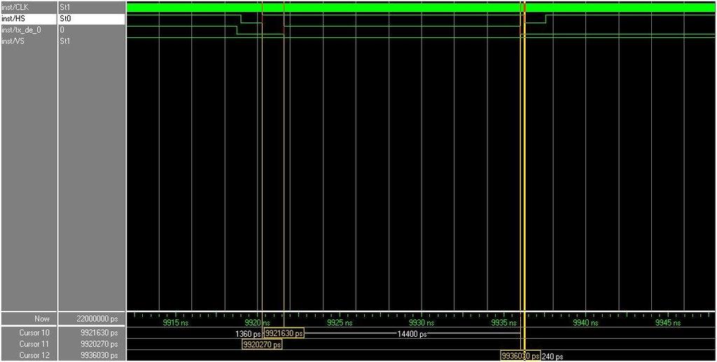
62 (a) (b) 56

63 (c) Figure 39: Simulation of Format Generator Module 2.4 Flow Control Module Table 9: Flow Control Module Interface Description Signal Direction Description Clk_c input clock input Reset_n input Reset signal, active low DE_c Input Data enable signal YUV_c[15:0] input Pixel data in YUV color space en_p output Vertical synchronization to transmitter en_fgen output Horizontal synchronization to transmitter YUV_p[15:0] output YUV data to processor core The function of this block is to detect the start of a frame, since the first data received can be an area in an image because the reset of the system may not happen during the vertical blank period. The VS signal has the information of the beginning of a frame, as shown in Figure 38. The simulation result is shown in Figure 39. The YUV_p output is equal to the YUV_c input, so the simulation does not include these two signals, the en_p and en_fgen in first prototype system are both the same as the en signal in Figure 39. Figure 39: Flow Control Simulation 2.5 Transmitter Module Table 10: Flow Control Module Interface Description Signal Direction Description Clk_t input clock input Reset_n input Reset signal, active low DE_t input Data enable signal from format generator HS_t input Horizontal synchronization from format generator VS_t input Horizontal synchronization from format generator YUV_t[15:0] input Pixel data in YUV color space clk_o Clock signal to display chip RGB_o[15:0] output Pixel data in RGB color space DE_o output Data enable signal to display chip HS_o output Horizontal synchronization to display chip 57