Inverse Filtering by Signal Reconstruction from Phase. Megan M. Fuller

Transcription

1 Inverse Filtering by Signal Reconstruction from Phase by Megan M. Fuller B.S. Electrical Engineering Brigham Young University, 2012 Submitted to the Department of Electrical Engineering and Computer Science in partial fulfillment of the requirements for the degree of Master of Science in Electrical Engineering and Computer Science at the MASSACHUSETTS INSTITUTE OF TECHNOLOGY June 2014 c Massachusetts Institute of Technology All rights reserved. Author Department of Electrical Engineering and Computer Science April 24, 2014 Certified by Jae S. Lim Professor of Electrical Engineering Thesis Supervisor Accepted by Professor Leslie A. Kolodziejski Chairman, Department Committee on Graduate Students

2 2

3 Inverse Filtering by Signal Reconstruction from Phase by Megan M. Fuller Submitted to the Department of Electrical Engineering and Computer Science on April 24, 2014, in partial fulfillment of the requirements for the degree of Master of Science in Electrical Engineering and Computer Science Abstract A common problem that arises in image processing is that of performing inverse filtering on an image that has been blurred. Methods for doing this have been developed, but require fairly accurate knowledge of the magnitude of the Fourier transform of the blurring function and are sensitive to noise in the blurred image. It is known that a typical image is defined completely by its region of support and a sufficient number of samples of the phase of its Fourier transform. We will investigate a new method of deblurring images based only on phase data. It will be shown that this method is much more robust in the presence of noise than existing methods and that, because no magnitude information is required, it is also more robust to an incorrect guess of the blurring filter. Methods of finding the region of support of the image will also be explored. Thesis Supervisor: Jae S. Lim Title: Professor of Electrical Engineering 3

4 4

5 Acknowledgments First, I would like to thank my advisor, Prof. Jae Lim, for giving me a place in his group. His support, patience, and insight have been invaluable, and he has helped me learn that most critical of research skills: How to ask questions. I would also like to thank my labmates, Xun Cai and Lucas Nissenbaum, for their help and friendship, and express my gratitude to Cindy LeBlanc, who keeps the group running. Finally, I am deeply indebted to my parents, who have always helped to cultivate my love of learning, and who have been such wonderful examples to me throughout my life. Thank you all. 5

6 6

7 Contents 1 Introduction 13 2 Background Image Restoration Magnitude Retrieval Performance in the Presence of Noise Effect of Noise on Phase Characterization of Phase-Based Deconvolution Experimental Setup Effect of the Number of Iterations Effect of the Size of the DFT Effect of the Starting Point Comparison to Other Methods Comparison to Inverse Filtering Techniques Comparison to Image Restoration Techniques Summary Performance with Imperfect Knowledge of the Blurring Function Attributes of Blurring Functions Characterization of Phase-Based Deconvolution Experimental Setup Effect of the Number of Iterations

8 4.2.3 Effect of the Size of the DFT Effect of the Starting Point Comparison to Other Methods Comparison to Inverse Filtering Techniques Comparison to Image Restoration Techniques Noise Characterization of Phase-Based Deconvolution Comparison to Other Methods Summary Obtaining the Region of Support Description of Methods ROS from the Degraded Image ROS from Morphological Processing ROS with Markers Comparison of Methods No Noise, Perfect Knowledge of the Blurring Function Noise, Perfect Knowledge of the Blurring Function No Noise, Imperfect Knowledge of the Blurring Function Summary Conclusions and Future Work 81 A Photo Credits 83 8

9 List of Figures 3-1 Original images OS-MSE as a function of noise variance and number of iterations for the tire image Example of artifacts present in the restored image when the algorithm was run to convergence Illustration of the effect of number of iterations on artifacts when stopping short of convergence was optimal Illustration of the effect of number of iterations on artifacts when convergence was optimal OS-MSE as a function of noise variance and DFT size for the cameraman image Illustration of the effect of DFT size on visual quality OS-MSE of the liftingbody image when the iteration was initialized with the degraded image magnitude OS-MSE of the bag image when the iteration was initialized with the undegraded image magnitude Comparison of deconvolution methods Cameraman image deconvolved with several different methods Comparison of restoration methods Cameraman image restored with several different methods Fourier transform of an 11x11-point Gaussian filter with σ = Comparison of the phases of two lowpass filters

10 4-3 OS-MSE of the bag image when the deblurring function was an 11x11- point averager Illustration of the artifacts produced in the bag image as the phasebased reconstruction iteration converged OS-MSE of the cameraman image when the deblurring function was an 11x11-point averager Illustration of the artifacts produced in the cameraman image as the phase-based reconstruction iteration converged OS-MSE of the liftingbody image when the deblurring function was an 11x11-point averager OS-MSE of the liftingbody image when the deblurring function was a 9x9-point averager Illustration of the effect of DFT size on visual quality when the deblurring filter was an 11x11-point averager OS-MSE as a function of number of iterations, DFT size, and starting point (constant and degraded magnitude) for the bag image OS-MSE as a function of number of iterations, DFT size, and starting point (constant and original magnitude) for two images OS-MSE as a function of number of iterations and DFT size for the liftingbody image (starting point degraded image) Comparison of inverse filtering techniques when the deblurring filter was an 11x11-point averager Comparison of inverse filtering techniques when the deblurring filter was a 9x9-point averager Comparison of restoration techniques when the deblurring filter was an 11x11-point averager Cell image restored with several different methods when the deblurring filter was an 11x11-point averager Cameraman image restored with several different methods when the deblurring filter was an 11x11-point averager

11 4-18 Comparison of restoration techniques when the deblurring filter was a 9x9-point averager Cameraman image restored with several different methods when the deblurring filter was a 9x9-point averager Comparison of phase-based deconvolution of the liftingbody image to existing methods (deblurring filter an 11x11-point averager) Liftingbody image restored with several different methods (deblurring filter an 11x11-point averager) Comparison of phase-based deconvolution of the liftingbody image to existing methods (deblurring filter a 9x9-point averager) Liftingbody image restored with several different methods (deblurring filter a 9x9-point averager) Original images used in the region of support experiments OS-MSE as a function of number of iterations and ROS error for the black moon image Illustration of the procedure used in marking a blurry image with an unknown region of support OS-MSE as a function of number of iterations and DFT size when the ROS was obtained by morphological processing Artifacts in convergent circle images OS-MSE as a function of number of iterations and DFT size when the ROS was obtained by the use of markers Artifacts in convergent images when markers were used to indicate the ROS Comparison of methods of determining the ROS of the black moon image in the presence of noise Comparison of artifacts produced by different methods of obtaining the ROS

12 5-10 OS-MSE of the circle image when the ROS and the size of the blurring function were unknown OS-MSE of the the black moon image when the ROS and the size of the blurring function were unknown

13 Chapter 1 Introduction Two-dimensional deconvolution is a problem of great practical interest. Images taken with a digital camera can be blurred by a number of sources, and often this blurring can be modeled as the convolution of the original image with a blurring function. Therefore, to obtain the original image from the degraded one requires a deconvolution. Many methods of doing this have been developed, each with its own strengths and weaknesses. Most of these methods rely on Fourier domain techniques. That is, they divide the Fourier transform of the degraded image by some function of the Fourier transform of the blurring function. This leads to two weaknesses in particular. First, because a blurring function is a lowpass signal, deconvolution in the frequency domain requires the high frequencies to be divided by very small numbers. Typical images are also lowpass signals, so this tends to amplify the noise in the image. Second, these methods rely on accurate knowledge of the blurring function. These weaknesses can be addressed by exploiting the fact that a typical image can be represented by only the phase of its Fourier transform and its region of support. This implies that only the phase of the Fourier transform of the image needs to be corrected and allows deconvolution to be performed by subtraction rather than division, thus mitigating the noise amplification problem. It also only requires knowledge of the phase of the Fourier transform of the blurring function, which may be easier to estimate in some situations than both the phase and the magnitude. 13

14 In this thesis, we will explore the strengths and weaknesses of doing deconvolution based on phase. In Chapter 2, the necessary background information will be presented, including the details of the deconvolution problem, a discussion of several existing deconvolution methods, and the algorithm by which an image can be reconstructed from only the phase of its Fourier transform and its region of support. In Chapter 3, we will examine the performance of phase-based deconvolution in the presence of noise. The effect of changing several parameters of the phasebased reconstruction algorithm will be explored and phase-based deconvolution will be compared to other methods. In Chapter 4, we will look at the performance of phase-based deconvolution when the blurring function is not known perfectly. The situations in which it is easier to estimate the phase of the Fourier transform of the blurring function than the entire Fourier transform of the blurring function will be explained. Again, the effect of changing the parameters of the phase-based reconstruction algorithm will be explored, and phase-based deconvolution will be compared to other methods. In Chapters 3 and 4, the region of support of the image will be assumed known. In Chapter 5, we will discuss and compare several methods for obtaining the region of support of the image if it is not known. Finally, in Chapter 6, we will conclude the thesis and suggest possible future work. 14

15 Chapter 2 Background This chapter will be divided into two parts. First, the image restoration problem will be explained, including a summary of some of the most common methods currently used to solve this problem. Then, a discussion of the magnitude retrieval problem will be presented. The way in which the magnitude retrieval problem relates to the image restoration problem is the topic of this thesis, and will be elaborated on in the next chapter. 2.1 Image Restoration Image degradation is typically modeled as a degradation system followed by additive noise [2]. Mathematically, this can be written as g(n 1, n 2 ) = f(n 1, n 2 ) b(n 1, n 2 ) + v(n 1, n 2 ) (2.1) or, in the frequency domain, G(ω 1, ω 2 ) = F (ω 1, ω 2 )B(ω 1, ω 2 ) + V (ω 1, ω 2 ) (2.2) where f(n 1, n 2 ) is the original image, b(n 1, n 2 ) is the degradation system, often some sort of blurring filter, v(n 1, n 2 ) is additive noise, which is known only in a statisti- 15

16 cal way, and g(n 1, n 2 ) is the degraded image. transforms of the respective sequences. Capital letters indicate the Fourier The goal of image restoration is to use g(n 1, n 2 ) and available information about f(n 1, n 2 ), b(n 1, n 2 ), and v(n 1, n 2 ) to compute some ˆf(n 1, n 2 ) that is an approximation of f(n 1, n 2 ). This notation will be used throughout. There are many variations on Eq For example, the additive noise could actually be data dependent, as in the case of Poisson noise, which is common in astronomical images [3]. It may be that the noise is not additive, but multiplicative, which is seen in infrared radar images [9]. However, one of the most common types of noise is signal independent additive white Gaussian. This fits the model of Eq. 2.1 and can come, at least approximately, from many sources, including the read out noise of A/D converters [3]. The blurring term, b(n 1, n 2 ), can also come from many sources. A few of the most common include lens misfocus, atmospheric turbulence, and uniform linear motion [9] [2]. Note that, in writing Eqs. 2.1 and 2.2, it was implicitly assumed that the blurring function was linear and space invariant. This is not always the case, but is approximately true for a large class of degradations and simplifies the restoration computations considerably [2]. Therefore, this assumption will remain in place. A host of methods currently exist to solve the image restoration problem, each with particular strengths and weaknesses. A few of the most common will now be explained. This list is not meant to be exhaustive, but representative of the kinds of algorithms available. Inverse Filtering: Inverse filtering involves the computation of ˆF (ω 1, ω 2 ) = G(ω 1, ω 2 ) B(ω 1, ω 2 ) (2.3) If B(ω 1, ω 2 ) is known perfectly and has no zeros, and if there is no noise, inverse filtering will produce exactly the correct answer. However, in the presence of noise, the noise can be amplified, and the result can become visually unacceptable [2]. Variations on inverse filtering include thresholded inverse filtering, where a maximum 16

17 value for 1 B(ω 1,ω 2 ) is set to avoid this problem [9] and the use of the pseudoinverse filter, which handles the problem of zeros in B(ω 1, ω 2 ) by setting ˆF (ω 1, ω 2 ) equal to zero at those points [7]. There are also iterative spatial domain methods to compute the deconvolution, and these can be stopped short of convergence or used to impose additional constraints (for example, non-negativity) on the final result [11]. It is worth emphasizing here that inverse filtering and its variations are a somewhat different class of algorithm from those explained below. Inverse filtering solves the problem of blurring, but makes no attempt to account for noise. The methods explained below were all designed with a specific noise model in mind and can be considered simultaneously deblurring and de-noising algorithms. Wiener Filtering: Wiener filtering consists of the computation of H(ω 1, ω 2 ) = 1 B(ω 1, ω 2 ) 2 B(ω 1, ω 2 ) B(ω 1, ω 2 ) 2 + S v (ω 1, ω 2 )/S f (ω 1, ω 2 ) (2.4) where S v (ω 1, ω 2 ) and S f (ω 1, ω 2 ) are the power spectral densities of the noise and signal, respectively. The image is then restored by taking the inverse Fourier transform of ˆF (ω 1, ω 2 ) = H(ω 1, ω 2 )G(ω 1, ω 2 ). The Wiener filter is often called the linear least mean squared error filter because it is a linear system and minimizes E{[f(n 1, n 2 ) ˆf(n 1, n 2 )] 2 } [2]. Whether this is the correct quantity to minimize will depend on the application. Unlike inverse filtering, Wiener filtering will not tend to amplify the noise. This can be seen by looking at Eq At frequencies where the noise is large relative to the signal, H(ω 1, ω 2 ) will be small, and at frequencies where the noise is small relative to the signal, H(ω 1, ω 2 ) will be large. However, Wiener filtering relies on knowledge of the power spectral densities of the signal and noise, and these may not be known precisely, if at all. Therefore, in practice, the approximation of Sv(ω 1,ω 2 ) S f (ω 1,ω 2 ) = K where K is some constant is often used [2]. There are many variations on the Wiener filter, including the parametric Wiener filter, which can give the user more control over the amount of smoothing done, and adaptive Wiener filters, which can account for spatial variance in the statistics of the 17

18 noise or image. These can give better results at the cost of more fine-tuning by the user or, in the case of adaptive Wiener filters, more computation [9]. Constrained Least Mean Squared Error Filter: Also known as the regularized filter, the constrained least mean squared error filter is an important variation of the Wiener filter that gives the minimum mean squared error solution under a constraint of minimizing the second derivative of the restored image. In this case, the deblurring filter is given by H(ω 1, ω 2 ) = 1 B(ω 1, ω 2 ) 2 (2.5) B(ω 1, ω 2 ) B(ω 1, ω 2 ) 2 + γ P (ω 1, ω 2 ) 2 where P (ω 1, ω 2 ) is the Laplacian operator, which serves as an approximation for the second derivative, and γ is a Lagrange multiplier. An optimum γ for given noise statistics can be found iteratively. Constraining the second derivative in this way tends to make the restored image smoother. This filter also has the advantage of not requiring any knowledge of the statistics of the signal or noise besides the mean and variance of the noise, which are used in the iteration to find γ [2]. Richardson-Lucy Iteration: The Richardson-Lucy iteration relies on a probabilistic interpretation of blurring. It treats the value of each pixel in f(n 1, n 2 ) as a count of the number of events that happened there. It assumes the blurring function is normalized, so that the total count of events in f(n 1, n 2 ) matches the total count of events in g(n 1, n 2 ). Then, it uses Bayes s theorem to find the probability of an event at a particular f(n 1, n 2 ) given an event at a particular g(n 1, n 2 ) and given the blurring function. It can be shown that the maximum likelihood solution to this problem can be found with the following iteration. (Note that the one-dimensional case is given for simplicity. The extension to two dimensions is straightforward.) f r+1 (i) = f r (i) f 0 (i) = c k=i n f(n) I b(k i + 1)g(k) d j=a b(k j + 1)f r(j) (2.6) (2.7) where I is the size of f(n), J is the size of b(n), a = max(1, k J + 1), d = min(k, I), 18

19 and c = i + J 1 [13]. Note that Eq. 2.7 is equivalent to ( ) g(n) f r+1 (n) = f r (n) b(n) b(n) f r (n) (2.8) where indicates correlation and indicates convolution [1]. The Richardson-Lucy iteration presents several advantages. It finds the maximum likelihood solution to the deconvolution problem subject to the constraint that the result be non-negative, and there is nothing in Eq. 2.7 which requires b(n 1, n 2 ) to be spatially invariant. Furthermore, bad pixels can be masked by simply not including them in the calculations [3]. However, if there is noise, the Richardson-Lucy iteration must be stopped short of convergence, or it will attempt to fit the noise too closely and produce unacceptable errors [10]. It is not a trivial matter to determine at what point the iteration should be stopped, and, depending on the features of the image, the optimal stopping point may be different for different regions [3]. There are many other image restoration methods. For example, several waveletbased techniques have recently been developed [8] [12]. The purpose of this section is not to give an exhaustive list of all possible algorithms. As will be explained in more detail in the next chapter, phase-based deconvolution is strictly an inverse filtering method. It will be compared to some image restoration methods not to imply that it should be used as a restoration system, but to demonstrate how robust it is. 2.2 Magnitude Retrieval The magnitude retrieval problem consists of reconstructing the magnitude of the Fourier transform of a signal given only the phase of the Fourier transform of that signal. Because any signal can be convolved with a zero-phase system and produce a different output with the same Fourier transform phase but a different magnitude, it is not, in general, possible to do this. However, it can be shown that if the Z-transform of the signal does not have any 19

20 zeros in conjugate-reciprocal pairs or on the unit circle, and if the region of support of the signal is known (that is, the signal is zero outside of some known range), then the signal is uniquely defined by the phase of its Fourier transform to within a scale factor [4]. These conditions can be extended to the case of multi-dimensional signals, and, furthermore, it can be shown that almost all two-dimensional signals satisfy the Z- transform domain constraints [4]. In addition, the phase of the continuous Fourier transform need not be known. The phase of a sufficiently large discrete Fourier transform (DFT) is also enough to uniquely identify the signal. In this case, a sufficiently large DFT for an image that is N 1 xn 2 pixels would be at least (2N 1 1)x(2N 2 1) points [4]. There is a closed-form solution to the problem of computing a spatial domain signal from the phase of its DFT. However, this requires the inversion of prohibitively large matrices when the signals are reasonably sized images. Fortunately, there is also an iterative algorithm which alternately imposes the spatial domain constraints and the frequency domain constraints [4]. Specifically, it is as follows, where x(n 1, n 2 ) is the signal to be reconstructed and X(k 1, k 2 ) is its DFT: 1. Start with an initial guess of the magnitude of X(k 1, k 2 ). Call this Y 0(k 1, k 2 ). This can be anything a constant, random values, the magnitude of the DFT of similar images, etc. The algorithm will converge from any starting point. 2. Compute Y r+1 (k 1, k 2 ) = Y r (k 1, k 2 ) e jθ X(k 1,k 2 ), where θ X (k 1, k 2 ) is the known phase of X(k 1, k 2 ). 3. Compute y r+1 (n 1, n 2 ) = IDFT[Y r+1 (k 1, k 2 )]. 4. Set y r+1(n 1, n 2 ) = y r+1 (n 1, n 2 ) inside the known region of support, and zero everywhere else. 5. Compute Y r+1(k 1, k 2 ) = DFT[y r+1(n 1, n 2 )]. 6. Repeat steps 2-5 until convergence is reached. 20

21 This algorithm has been proven to converge to the correct solution, provided the uniqueness constraints are met [4]. This algorithm works with general twodimensional signals. In the special case of images, when the values of the spatial domain signal are known to be positive, step 4 can be modified to set y r+1(n 1, n 2 ) = y r+1 (n 1, n 2 ) inside the region of support, and the algorithm will still converge [14]. 21

22 22

23 Chapter 3 Performance in the Presence of Noise 3.1 Effect of Noise on Phase The relationship between white Gaussian noise in the spatial domain and phase errors in the Fourier transform of a signal is quite complicated. Any particular sample of the Fourier transform is a function of all the spatial domain samples, leading to a large covariance matrix. Furthermore, in the case of real, finite-length signals, such as images, the real and imaginary parts of the Fourier transform are not independent, but related by the Hilbert transform. Finally, the phase is the arctangent of the imaginary part divided by the real part, which is a nonlinear operation. This makes it very difficult to perform any theoretical analysis of the phase of white noise, even before the signal has been added to it. Furthermore, because the noise model being considered is additive, the phase of the signal and the phase of the noise do not interact in a straightforward way. Instead, the phase of the noisy signal is given by θ G (ω 1, ω 2 ) = tan 1 ( ) Im{F (ω 1, ω 2 )} + Im{V (ω 1, ω 2 )} Re{F (ω 1, ω 2 )} + Re{V (ω 1, ω 2 )} (3.1) where G(ω 1, ω 2 ) is the Fourier transform of the noisy signal, θ G (ω 1, ω 2 ) is the phase 23

24 of G(ω 1, ω 2 ), F (ω 1, ω 2 ) is the Fourier transform of the original signal, and V (ω 1, ω 2 ) is the Fourier transform of the noise. Qualitatively, this means that, where the real or imaginary parts of F (ω 1, ω 2 ) are large relative to V (ω 1, ω 2 ), the effect of the noise on the phase will be small, and where the real or imaginary parts of the signal are small relative to the noise, the effect on the phase will be large. 3.2 Characterization of Phase-Based Deconvolution For the same reasons it is difficult to perform a theoretical analysis of spatial domain noise on the Fourier transform of a signal, it is also difficult to analyze what noise in the phase of the Fourier transform of a signal will do to the reconstructed signal. However, noise in the phase does not seem to change the fact of convergence of the algorithm to some solution. What this convergent solution is depends on the size of the internal DFT used by the iteration and the starting point of the iteration. Additionally, the question remains whether the convergent solution is the best representation of the original image, or whether it would be better to stop the iteration at some intermediate point, as is the case with the Richardson-Lucy iteration. In this section, we will first explain the experimental setup used to produce the reported results. We will then examine the effect of the number of iterations, the effect of the size of the internal DFT used in the iteration, and the effect of the starting point of the iteration Experimental Setup These experiments were performed assuming the basic model of image degradation held. That is, g(n 1, n 2 ) = f(n 1, n 2 ) b(n 1, n 2 ) + v(n 1, n 2 ) (3.2) 24

25 where many different images were used for f(n 1, n 2 ), b(n 1, n 2 ) was an 11x11-point Gaussian filter with σ = 5, and v(n 1, n 2 ) was zero-mean Gaussian white noise with differing variances. The images used are shown in Fig These cover a variety of image characteristics, and the results can be considered representative. Note that, while the original image aspect ratios have been preserved in Fig. 3-1, the original sizes have not. For example, the original cameraman image was 256x256 pixels, while the original liftingbody image was 512x512 pixels, even though these two appear to be the same size in Fig Also, Fig. 3-1a, 3-1c, and 3-1i are shown at 75% their true resolution for copyright reasons. (See Appendix A for image credits.) In this chapter, the blurring function and the region of support were assumed known. The effect of loosening these assumptions will be addressed in subsequent chapters. The quality metric used was a variation of mean squared error, computed as e = 1 N 1 N 2 N 1 1 N 2 1 n 1 =0 n 2 =0 ( f(n 1, n 2 ) k ˆf(n 1, n 2 )) 2 (3.3) where k is a scale factor computed to minimize the error, and is given by k = N1 1 N2 1 n 1 =0 N1 1 n 1 =0 n 2 =0 f(n 1, n 2 ) ˆf(n 1, n 2 ) ( 2 (3.4) ˆf(n1, n 2 )) N2 1 n 2 =0 This metric, which will be referred to as optimal scaling mean squared error (OS- MSE), was chosen because phase-based reconstruction is only accurate to within a scale factor. It should be noted that the original image would not typically be available in practice, and so k would have to be estimated. It should also be noted that this error measure is not necessarily an absolute indicator of visual quality, and so sample images will be provided throughout to demonstrate the kinds of artifacts present in the restored images. Unless stated otherwise, the initial guess of the magnitude of the restored image used by the phase-based reconstruction iteration was simply a constant. In some cases, the phase-based reconstruction iteration led to an intermediate spatial domain 25

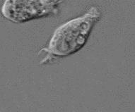
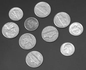
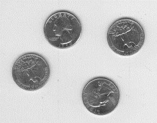
26 (a) moon (358x537 pixels) (b) bag (189x250 pixels) (c) pout (240x291 pixels) (d) cameraman (256x256 pixels) (e) liftingbody (512x512 pixels) (f) tire (232x205 pixels) (g) circuit (272x280 pixels) (h) westconcordorthophoto (364x366 pixels) (i) rice (256x256 pixels) (j) cell (191x159 pixels) (k) coins (300x246 pixels) (l) eight (308x242 pixels) Figure 3-1: Original images 26

27 image with such small pixel values that the quantization of double precision floatingpoint numbers became a problem. To avoid this, a check was placed in the iteration to multiply the reconstructed image by a large constant if it ever became too small. Since phase-based reconstruction only gives the result to within a scale factor, this would not change the final result. The alternative would be to compute and scale by k at each iteration. This was not done to avoid introducing any dependence on the original f(n 1, n 2 ) into the iteration Effect of the Number of Iterations To find the optimal number of iterations, the original image was degraded as described previously and the phase-based reconstruction algorithm was allowed to run for a certain number of iterations. The OS-MSE between the resulting restored image and the original was computed and saved. This was repeated for several different amounts of noise, for different DFT sizes, and for each image. In almost every case, more iterations improved the quality of the restored image in the OS-MSE sense until convergence was reached. The results for the tire image with an internal DFT size of twice the image size, shown in Fig. 3-2, were typical. Convergence was found to occur between 500 and 1,000 iterations in general, with the notable exception being the moon image, which was still improving after even 10,000 iterations. It should be emphasized that there is no theoretical guarantee of convergence in the presence of noise, but all the experiments in this chapter did indeed find some convergent solution except the moon image, which also seemed to be converging even though the experiments were not run long enough to actually reach convergence. The few cases in which more iterations did not always lead to a lower OS-MSE were the bag, westconcordorthophoto, and coins images at low noise values and the cell image at high noise values. In the case of the bag, westconcordorthophoto, and coins images, the visual quality of the convergent solutions was similar to that of the preconvergent solutions, and which was considered the better restoration would probably be a matter of application. 27

28 iters 100 iters 500 iters 1000 iters 2000 iters 500 OS MSE noise variance Figure 3-2: OS-MSE as a function of noise variance and number of iterations for the tire image. Internal DFT size was twice the image size. There are several things to note about this analysis. First, the kind of artifacts that appeared in the convergent solution, namely horizontal and vertical lines, was similar across all images. A few examples are shown in Fig The preconvergent solutions showed varying artifacts, but graininess was common. As convergence was reached, these artifacts tended to be diminished and the horizontal and vertical lines became better defined. In some cases, the convergent solution appeared somewhat less sharp than the preconvergent solution. A few examples of this are shown in Figs. 3-4 and 3-5. In these and all subsequent restored images, only the region of support of the original image is shown the degraded image was slightly larger because of the blurring. From these results, it is reasonable to conclude that, in general, phase-based deconvolution performs best when run to convergence. Even when this is not the 28

29 (a) liftingbody, restored (b) cell, restored Figure 3-3: Example of artifacts present in the restored image when the algorithm was run to convergence. Noise variance was 1. (a) 500 iterations (b) 1000 iterations (c) 2000 iterations Figure 3-4: An illustration of the effect of number of iterations on artifacts when stopping short of convergence was optimal. As the number of iterations increases, the lines surrounding the coins decrease and the image becomes less sharp. In this case, the restored image has a slightly higher OS-MSE as the number of iterations increases, but the visual quality is not clearly worse. Noise variance was

30 (a) 50 iterations (b) 100 iterations (c) 500 iterations Figure 3-5: An illustration of the effect of number of iterations on artifacts when convergence was optimal. As the number of iterations increases, the graininess decreases and the horizontal and vertical lines become more pronounced. Noise variance was 1. case in the OS-MSE sense, it may be in the visual quality sense, and any gains to be had by stopping short of convergence are small Effect of the Size of the DFT In the absence of noise, there is one correct solution, and the phase-based reconstruction iteration will converge to that solution regardless of the size of the internal DFT, provided it is at least twice the image size, as required by the uniqueness theorem. In the presence of noise, however, a solution that satisfies both the spatial and frequency domain constraints simultaneously may not exist. In this case, convergence indicates a point has been found such that the spatial and frequency constraints are being violated circularly. That is, a frequency domain solution, when corrected with the given phase, produces a spatial domain solution, that, when corrected with the given region of support, has a Fourier transform equal to the original frequency domain solution, and the progress of the algorithm stops. If this is the situation, then the size of the DFT used by the phase-based reconstruction algorithm could change the solution to which the reconstruction algorithm converges. This does seem to be the case in practice. The images were restored with DFT sizes of 2, 3, 4, and 5 times the corrupted image size. These tests produced no clear winner among the DFT sizes, though in general a DFT size of twice the image size did somewhat worse than the others, and a size of five times the image size often did 30

31 dft size 2 dft size 3 dft size 4 dft size OS MSE noise variance Figure 3-6: OS-MSE as a function of noise variance and DFT size for the cameraman image. Here dft size 2 indicates the internal DFT size was twice the degraded image size, dft size 3 indicates three times the degraded image size, and so forth. Results are the convergent solution. somewhat better. However, the differences were only slight, and it seems there is not much to be gained by changing the DFT size. The cameraman image was typical, and the results are shown in Figs. 3-6 and 3-7. Fig. 3-6 shows the OS-MSE values of the convergent solutions of each DFT size, and Fig. 3-7 shows the actual images. Careful inspection does indicate that a size of 3, 4, or 5 times the image size is somewhat better than twice the image size, but the gains are small. Nevertheless, phase-based deconvolution is computationally intensive regardless of the DFT size and will be most useful in situations where computational power is not an issue. This being the case, there is no reason not to use a larger DFT to capture whatever gains are available. 31

32 (a) DFT size: twice the image size (b) DFT size: three times the image size (c) DFT size: four times the image size (d) DFT size: five times the image size Figure 3-7: Illustration of the effect of DFT size on visual quality. Noise variance was Effect of the Starting Point Although the previous experiments were performed with a constant as the initial guess of the image magnitude, there is no reason this must be the case. In the absence of noise, the algorithm will eventually converge to the correct solution from any non-zero starting point, and, in the presence of noise, the starting point may affect the solution to which the iteration converges. A constant is one convenient choice, but there are other natural options. For example, the starting point could be the magnitude of the degraded image. Experiments performed from this starting point gave, in general, very similar convergent results to those produced by the previous experiments. Improvements 32

33 achieved by changing the starting point were slight, and which starting point was better was a function of both the image being restored and the noise level with which it was corrupted, with no clear pattern emerging. The exception to this rule was the moon image, where the results obtained by starting with the degraded image were much better than those obtained by starting with a constant. This is likely because the phase-based reconstruction algorithm did not reach convergence from either starting point. It was frequently the case that the preconvergent solutions obtained by starting with the degraded image were better than those obtained by starting with a constant, even though the convergent results were similar and the starting point did not seem to affect how many iterations were required for convergence. The general trends that held when the starting point was a constant also held when the starting point was the degraded image. That is, the convergent solution was typically the best and an internal DFT size of at least three times the degraded image size frequently did better than an internal DFT size of only twice the degraded image size. There were, however, several situations in which these general rules did not hold. For example, in some of the images, at high noise values, fewer iterations became better than the convergent solution. This is likely because the phase was sufficiently noisy and the initial guess of the magnitude was sufficiently accurate that attempting phase-based reconstruction of the magnitude actually produced a magnitude that was more corrupted than the original. The liftingbody image was representative of this class, and results are shown in Fig This was further confirmed by experiments in which the original, undegraded image magnitude was used as the starting point. In this case, fewer iterations always gave a better result. A particularly dramatic example of this was the bag image. The results are shown in Fig Again, this is reasonable a correct initial magnitude can only be corrupted by a noisy phase during reconstruction. (Interestingly, the convergent solution was comparable to that obtained when starting with a constant or the degraded image.) From this, it is reasonable to conclude that, if the phase-based reconstruction 33

34 iters 100 iters 500 iters 1000 iters 2000 iters 200 OS MSE noise variance Figure 3-8: OS-MSE as a function of noise variance and number of iterations for the liftingbody image when the iteration was initialized with the degraded image magnitude. The internal DFT size was twice the image size. iteration is run to convergence, the starting point doesn t matter. However, if a sufficiently accurate initial guess of the magnitude is paired with a sufficiently noisy phase, there are some gains to be had by stopping before convergence, though what is sufficiently accurate and sufficiently noisy will have to be determined in an ad-hoc manner and may require some trial and error. Additionally, if, because of computing constraints, the iteration cannot be run to convergence, starting with the degraded image will likely give a better result and is the recommended procedure. In light of this, the remainder of this chapter will continue to use results obtained from a constant initial magnitude. Though in certain situations some ad-hoc improvements may be possible, these will not be explored. The focus of the discussion is on what can be achieved based on phase information, and starting with a constant both eliminates the need for magnitude information and provides a consistent starting 34

35 iters 100 iters 500 iters 1000 iters 2000 iters 800 OS MSE noise variance Figure 3-9: OS-MSE as a function of noise variance and number of iterations for the bag image when the iteration was initialized with the undegraded image magnitude. The internal DFT size was twice the image size. point for all images. 3.3 Comparison to Other Methods Phase-based deconvolution is, strictly speaking, an inverse filtering technique and not an entire image restoration system. That is to say, it makes no attempt to account for or correct noise in the image. Therefore, the proper comparison is to other inverse filtering techniques. However, phase-based deconvolution has proven to be so robust in the presence of noise that it can also be compared to full image restoration algorithms that do account for noise. The methods included in these comparisons are not an exhaustive list of the possibilities there are far too many algorithms. The comparisons provided are only 35

36 meant to serve as a dramatic demonstration of the result that phase-based deconvolution is extremely robust to noise. They do not imply that phase-based deconvolution should be used as an image restoration system. In all cases, the phase-based reconstruction iteration was initialized with a constant and run to convergence with an internal DFT that was five times the degraded image size Comparison to Inverse Filtering Techniques There were three inverse filtering methods considered, namely: Direct Inverse Filtering, simply the inverse DFT of the N 1 xn 2 point DFT of the degraded image divided by the N 1 xn 2 point DFT of the blurring filter, where the degraded image was N 1 xn 2 pixels. Thresholded Inverse Filtering, where the inverse filter was limited to have a magnitude of no more than 1, 000 at all points. No Processing, where no processing was performed on the degraded image. Phase-based deconvolution performed much better than either direct or thresholded inverse filtering in all cases, and was usually better than doing no processing, though at high noise levels the moon, pout, liftingbody, cell, and eight images were slightly better left alone. (The moon image had not reached convergence when the test ended, and so further improvement was probably possible if it had been allowed to run for more iterations.) The results for the cameraman and eight images were typical and are shown in Fig Visual artifacts in the camerman image are shown in Fig Comparison to Image Restoration Techniques The results of phase-based deconvolution will now be compared with the results given by several methods of image restoration as a further demonstration of phase-based deconvolution s robustness in the presence of noise. The methods used are Wiener Filtering, with the power spectral densities of the noise and signal assumed 36

37 x inverse thresholded inverse no processing phase based inverse thresholded inverse no processing phase based OS MSE OS MSE noise variance (a) cameraman noise variance (b) eight Figure 3-10: Comparison of deconvolution methods to be constants, so that Sv(ω 1,ω 2 ) S f (ω 1,ω 2 ) was just the noise to signal ratio. Noise statistics were assumed known and the noise to signal ratio was estimated from the corrupted image. Regularized Filtering, with the noise statistics assumed known and the Laplacian operator used for smoothing. Richardson-Lucy Iteration, taking into account white noise, with the noise statistics assumed known. The original (undegraded) image was used to determine the first local minimum in OS-MSE as a function of the number of iterations for each situation, and that number of iterations was used for that situation. In general, phase-based deconvolution did better than Wiener filtering and was comparable to the Richardson-Lucy iteration and regularized filtering in the OS-MSE sense at low noise values. It tended to do somewhat worse than the other methods at high noise values. The results for the liftingbody, cameraman, and bag images, shown in Fig. 3-12, were representative. Visual quality tracked OS-MSE fairly well in this test, but different restoration methods produced different artifacts, and which artifacts were considered most unpleasant would probably depend on the application. typical, and some sample images are shown in Fig The cameraman image was It is worth emphasizing again that, unlike phase-based deconvolution, all other methods require some knowledge of the noise statistics. Because other methods try to 37

38 (a) no processing (b) direct inverse filtering (c) thresholded inverse filtering (d) phase-based deconvolution Figure 3-11: Cameraman image deconvolved with several different methods. Noise variance was correct for the presence of noise and phase-based deconvolution does not, phase-based deconvolution is most competitive at high signal to noise ratios and becomes worse as the noise increases. Additionally, it should be noted that the original image was used to determine how long the Richardson-Lucy iteration should run. In practice, the original image would not be available and the number of iterations would have to be estimated. This means that results from that iteration will not typically be quite as good as shown here. 38

39 Wiener regularized phase based Richardson Lucy Wiener regularized phase based Richardson Lucy OS MSE OS MSE noise variance noise variance (a) liftingbody (b) cameraman Wiener regularized phase based Richardson Lucy 800 OS MSE Summary noise variance (c) bag Figure 3-12: Comparison of restoration methods In this chapter, we have shown that phase-based deconvolution is robust to the presence of noise. When initialized with a constant, the phase-based reconstruction iteration performs best when run to convergence, though there are minor exceptions to this rule. Larger internal DFT sizes also tend to perform better. There are some ad-hoc gains possible if a noisy enough phase is paired with an accurate enough estimate of the magnitude and the iteration is stopped short of convergence, but these may be hard to realize in practice. Phase-based deconvolution performs much better than other deconvolution methods in the presence of noise, and is competitive with restoration methods at low noise levels. 39

40 (a) degraded (b) direct inverse filtering (c) Wiener filtering (d) regularized filtering (e) Richardson-Lucy iteration (f) phase-based deconvolution Figure 3-13: Cameraman image restored with several different methods. Noise variance was 1. 40

41 Chapter 4 Performance with Imperfect Knowledge of the Blurring Function 4.1 Attributes of Blurring Functions Blurring functions are, by definition, two-dimensional lowpass filters. Additionally, a large class of blurring functions are symmetric (for example, those caused by lens misfocus [9]), and so their phases are limited to 0 or π. Among such functions, the Fourier transforms are sync-like. For example, the 512x512-point Fourier transform of an 11x11-point Gaussian filter with σ = 5 (the blurring function used in the previous chapter) is shown in Fig It is generally the case with such functions that the number of points in the filter determines the width of the main lobe, while the shape, or taper, of the filter merely changes the height of the side lobes. This has significant implications for the phase of the Fourier transforms of such filters. Specifically, the phases of two filters that are the same size will be very similar regardless of their respective tapers. This is illustrated dramatically in Fig. 4-2, which shows an 11x11-point Guassian filter with σ = 5, an 11x11-point averaging filter, and the difference between the phases of their 41

42 Figure 4-1: Fourier transform of an 11x11-point Gaussian filter with σ = 5 Fourier transforms. In practice, situations arise in which the blurring function is not known perfectly, but a reasonable guess can be obtained. Because of the similarity in phase across many different blurring functions of the same size, it seems likely that phase-based deconvolution will be fairly robust to imperfect knowledge of the blurring function. In the remainder of this chapter, we will characterize the performance of phasebased deconvolution when the blurring function is known imperfectly and compare phase-based deconvolution to other deconvolution and restoration methods. 4.2 Characterization of Phase-Based Deconvolution Experimental Setup The experimental setup in this chapter will be similar to that described in Chapter 3. Initially, the additive noise will be assumed to be zero so the effects of an incorrect 42

43 (a) 11x11-point Gaussian filter with σ = 5 (b) 11x11-point averaging filter (c) Difference in the angles of the 512x512-point Fourier transforms of the two filters. Blue regions indicate the angles were the same, while red indicates they differed by π. Figure 4-2: Comparison of the phases of two lowpass filters guess of the blurring function can be seen clearly. Noise will be added in again at the end of the chapter to increase the realism of the model. The reference images of Fig. 3-1 will still be used and the blurring function will still be the 11x11-point Gaussian filter with σ = 5. As in Chapter 3, the region of support will be assumed known and the error criterion will be the optimal scaling mean squared error defined in Eqs. 3.3 and 3.4. There will be two deblurring functions considered: An 11x11-point averager and a 9x9-point averager. These were chosen because an averager, being a constant over its region of support, is the simplest blurring function possible, and therefore would 43

44 be a natural initial guess of an unknown blurring function. Comparing the results obtained with these two averagers will also serve to highlight the relative importance of the size of the blurring function and the relative unimportance of its taper to phase-based deconvolution. All blurring and deblurring functions considered will be centered at the origin. Any shift in the blurring function away from the origin merely introduces a linear phase term, which, assuming it is known, can be easily accounted for after deconvolution. As in Chapter 3, the effect of the number of iterations, size of the internal DFT, and starting point will be considered in turn. It is necessary to run these experiments again because in Chapter 3 the errors in the phase were of random size and direction, having the greatest effect on those frequencies for which the signal to noise ratio of the degraded image was low. In contrast, when the errors in phase are due to imperfect knowledge of the blurring function, they will be fewer but more dramatic (those phases which are wrong will be wrong by π) and occur in a pattern determined by the blurring and deblurring functions. There is, therefore, no particular reason to expect the results of Chapter 3 to hold Effect of the Number of Iterations As with noisy signals, there is no theoretical guarantee of convergence when the deblurring filter is not the same as the blurring filter. However, all the experiments in this chapter did exhibit convergent behavior. Unlike the results obtained from signals corrupted with additive white Gaussian noise, however, the convergent solution was not always the optimal solution. When the deblurring filter was an 11x11-point averager, the preconvergent solutions were often sharper than the convergent solutions, though they were also grainier and had more pronounced ringing. Whether the effect of the increased sharpness or the effect of the increased graininess and ringing dominated depended on the image being restored. In the case of the moon, pout, liftingbody, circuit, coins, and eight images, the convergent solution was the best in the OS-MSE sense. For the other images, there was a preconvergent solution, typically around a few hundred iterations, 44

45 dft size 2 dft size 3 dft size 4 dft size OS MSE number of iterations Figure 4-3: OS-MSE as a function of number of iterations and DFT size for the bag image when the deblurring function was an 11x11-point averager that was at least slightly better than the convergent solution in the OS-MSE sense. The bag image was the most dramatic example of a preconvergent solution being better than a convergent solution, and results are shown in Figs. 4-3 and 4-4. (The effects of different DFT sizes will be discussed in the next subsection, and only the curve corresponding to an internal DFT size of twice the image size in Fig. 4-3 need be considered here.) The results for the cameraman image were more typical and are shown in Figs. 4-5 and 4-6. The liftingbody image was representative of the images for which the convergent solution was the best, and results are shown in Fig When the deblurring filter was a 9x9-point averager, there was an optimal preconvergent solution for the pout, cell, coins, eight, and tire images. As expected, in all cases the results were worse than what was obtained when using an averager of the correct size. The liftingbody image was representative of those images for which the convergent solution was optimal, and the results are shown in Fig

46 (a) degraded image (b) restored with 100 iterations (best solution) (c) restored with 1000 iterations (convergent solution) Figure 4-4: Illustration of the artifacts produced in the bag image as the phase-based reconstruction iteration converged when the blurring filter was an 11x11-point Gaussian, σ = 5 and the deblurring filter was an 11x11-point averager. In this example, a preconvergent solution is optimal. Internal DFT size was twice the image size dft size 2 dft size 3 dft size 4 dft size OS MSE number of iterations Figure 4-5: OS-MSE as a function of number of iterations and DFT size for the cameraman image when the deblurring function was an 11x11-point averager 46

47 (a) degraded image (b) restored with 300 iterations (best solution) (c) restored with 1500 iterations (convergent solution) Figure 4-6: Illustration of the artifacts produced in the cameraman image as the phase-based reconstruction iteration converged when the blurring filter was an 11x11-point Gaussian, σ = 5 and the deblurring filter was an 11x11-point averager. In this example, a preconvergent solution is optimal. Internal DFT size was twice the image size dft size 2 dft size 3 dft size 4 dft size OS MSE number of iterations Figure 4-7: OS-MSE as a function of number of iterations and DFT size for the liftingbody image when the deblurring function was an 11x11-point averager 47

48 1500 dft size 2 dft size 3 dft size 4 dft size OS MSE number of iterations Figure 4-8: OS-MSE as a function of number of iterations and DFT size for the liftingbody image when the deblurring function was a 9x9-point averager These results lead to several observations. First, if the texture of the original image is unknown, it will be difficult to determine to what extent the graininess in the restored image (in either the convergent or preconvergent solutions) is an artifact of restoration. Therefore, it may be difficult to know when to stop the iteration for an optimal result. Relatedly, this may be a situation in which OS-MSE is not necessarily an accurate indicator of visual quality. The correct balance of image sharpness and graininess or ringing is really a matter of application, and so OS-MSE is only a coarse indicator of quality. Nevertheless, when the deblurring filter was the correct size, both the preconvergent and convergent restored images were much sharper and showed much more detail than the blurred image itself. This indicates that it would be reasonable, when dealing with uncertainty in the taper of the blurring function, to run the phase-based 48

49 deconvolution algorithm for a few different numbers of iterations (including one that produces the convergent solution) and choose the result that looks the best. While this procedure is unlikely to produce the optimal solution in the OS-MSE sense, it is very likely to give a result that is better than the degraded image Effect of the Size of the DFT When the deblurring filter was either an 11x11-point or a 9x9-point averager, the size of the DFT used by the iteration did not have much of an effect on the final result. As a general trend, a larger DFT size was slightly better, and the most dramatic jump was from a DFT size of twice the degraded image size to a DFT of three or more times the image size, as illustrated in Figs. 4-7 and 4-8. The corresponding restored images when the deblurring filter was an 11x11-point averager are shown in Fig Careful inspection does reveal some slight variations in the ringing patterns, but, above a DFT size of twice the image size, it is difficult to say which is the best solution, though by OS-MSE, quality does improve with size in this case. Again, phase-based deconvolution is computationally intensive regardless of the DFT size and will be most useful in situations where computational power is not an issue. This being the case, there is no reason not to use a larger DFT size to capture whatever gains are available Effect of the Starting Point Experiments performed with the degraded image as the starting point for the phasebased deconvolution iteration yielded some interesting results when the deblurring filter was an 11x11-point averager. In every case but the cell image, more iterations led to a lower error, so the convergent solution was always the best. Additionally, for any given internal DFT size, the iteration converged to the same solution whether it was initialized with a constant or with the degraded image. These two observations together indicate the potential gains from stopping the iteration early when it is started with a constant cannot be realized when it is started with the degraded image. 49

50 (a) DFT size: twice the image size (b) DFT size: three times the image size (c) DFT size: four times the image size (d) DFT size: five times the image size Figure 4-9: Illustration of the effect of DFT size on visual quality when the deblurring filter was an 11x11-point averager. Images correspond to the the convergent solutions. 50

51 init const dft size 2 init const dft size 3 init const dft size 4 init const dft size 5 init deg dft size 2 init deg dft size 3 init deg dft size 4 init deg dft size OS MSE number of iterations Figure 4-10: OS-MSE as a function of number of iterations, DFT size, and starting point for the bag image. Starting points used are a constant ( init const ) and the degraded image magnitude ( init deg ). The deblurring filter was an 11x11-point averager. Notice how, for any given DFT size, the solutions converge to the same answer, regardless of starting point. These features are illustrated in Fig Because the convergent solutions are the same and the preconvergent gains are unavailable when starting with the degraded image, there seems to be no advantage to doing so. When the correct image magnitude was used as the starting point, it was almost always the case that a low number of iterations (about 100 or less) gave the best results. This is likely the same effect seen with the deconvolution of noisy images: An accurate enough estimate of the magnitude is only corrupted by attempting phasebased reconstruction with a noisy enough phase. Interestingly, the convergent solutions were again the same as those obtained when starting with a constant, though convergence was typically reached much sooner. This is illustrated in Fig Results were similar when the deblurring filter was a 9x9-point averager, but, when the degraded image magnitude was used as the starting point, fewer iterations were better for the cell and eight images, and the optimal number of iterations depended 51

52 init const dft size 2 init const dft size 3 init const dft size 4 init const dft size 5 init orig dft size 2 init orig dft size 3 init orig dft size 4 init orig dft size OS MSE number of iterations (a) bag init const dft size 2 init const dft size 3 init const dft size 4 init const dft size 5 init orig dft size 2 init orig dft size 3 init orig dft size 4 init orig dft size 5 OS MSE number of iterations (b) westconcordorthophoto Figure 4-11: OS-MSE as a function of number of iterations, DFT size, and starting point for the bag and westconcordorthophoto images. Starting points used are a constant ( init const ) and the original image magnitude ( init orig ). The deblurring filter was an 11x11-point averager. 52

53 dft size 2 dft size 3 dft size 4 dft size 5 OS MSE number of iterations Figure 4-12: OS-MSE as a function of number of iterations and DFT size for the liftingbody image. The starting point was the degraded image magnitude and the deblurring filter was a 9x9-point averager. on the DFT size for the pout and liftingbody images, as shown in Fig (This was also seen in the liftingbody image when the deblurring filter was an 11x11-point averager and the undegraded image magnitude was used as the initial magnitude.) Again, the convergent solutions always matched what was obtained when the initial magnitude was a constant. When the deblurring filter was a 9x9-point averager and the starting point was the magnitude of the undegraded image, a low number of iterations (a few hundred or less) was almost always best. The one exception was the cameraman image, which improved with increasing iterations until convergence was reached. Again, the iteration converged to the same value as it did when the initial magnitude was a constant. These results indicate that, if the algorithm is run to convergence, the starting point doesn t matter. However, there are gains to be had if an accurate enough 53

54 estimate of the magnitude is used as the starting point and the iteration is stopped short of convergence. What constitutes accurate enough is difficult to say, but it often must be better than the degraded image itself, and so such an estimate is not likely to be available and the iteration should simply be started with a constant initial value. 4.3 Comparison to Other Methods As in Chapter 3, phase-based deconvolution will now be compared first with other inverse filtering techniques and then with image restoration techniques. In all cases, the phase-based deconvolution iteration was initialized with a constant and used an internal DFT size of five times the size of the degraded image. Because there were situations in which stopping the iteration short of convergence was advantageous, both the best (to within 100 iterations) and the convergent solution will be presented in the comparisons Comparison to Inverse Filtering Techniques The same inverse filtering methods considered in Chapter 3 will be used here, namely inverse filtering, thresholded inverse filtering (which prevents the inverse filter from exceeding a magnitude of 1, 000), and doing no processing. The results of this comparison when the deblurring filter was an 11x11-point averager are shown in Fig The results for a 9x9-point averager are shown in Fig From these results, it can be seen that phase-based deconvolution was much more robust to errors in the deblurring function than either direct or thresholded inverse filtering, and was almost always an improvement on doing nothing, regardless of whether the iteration was run to convergence or stopped at an optimal point before. As expected, when the deblurring filter was a 9x9-point averager, the results of phase-based deconvolution were worse than when the deblurring filter was an 11x11- point averager. However, even in this case the restored image was often better than the degraded image. 54

55 inverse limited inverse no processing phase based (best) phase based (convergent) OS MSE bag cameraman cell circuit coins eight liftingbody pout rice tire westconcord moon image (a) Comparison of inverse filtering techniques inverse limited inverse no processing phase based (best) phase based (convergent) 1000 OS MSE bag cameraman cell circuit coins eight liftingbody pout rice tire westconcord moon image (b) Fig. 4-13a rescaled to highlight phase-based deconvolution Figure 4-13: Comparison of inverse filtering techniques when the blurring filter was an 11x11-point Gaussian with σ = 5 and the deblurring filter was an 11x11-point averager 55

56 inverse limited inverse no processing phase based (best) phase based (convergent) OS MSE bag cameraman cell circuit coins eight liftingbody pout rice tire westconcord moon image (a) Comparison of inverse filtering techniques inverse limited inverse no processing phase based (best) phase based (convergent) 1000 OS MSE bag cameraman cell circuit coins eight liftingbody pout rice tire westconcord moon image (b) Fig. 4-14a rescaled to highlight phase-based deconvolution Figure 4-14: Comparison of inverse filtering techniques when the blurring filter was an 11x11-point Gaussian with σ = 5 and the deblurring filter was a 9x9-point averager 56

57 4.3.2 Comparison to Image Restoration Techniques Again, the same image restoration algorithms used in Chapter 3 will be used here, namely Wiener filtering, regularized filtering, and the Richardson-Lucy iteration. In this case, there arises some ambiguity in what to use for the noise parameters input to the Wiener and regularized filters. There is no noise in the degraded image. However, there is some noise in the restoration in the incorrect guess of the blurring function. This noise is difficult to describe without knowledge of the correct blurring function, which obviously isn t available. Therefore, it is incorrect to say there is no noise when using the Wiener and regularized filters, but what is correct to say instead is ambiguous. For the purposes of these experiments, the noise used was simply Gaussian noise with a low, arbitrary variance. This is certainly not the right answer. However, it did achieve the desired effect of causing the Wiener and regularized filters to behave as though there was some low level of noise in the system. The performance of these algorithms could likely be improved with a better description of the noise, but a better description of the noise is equivalent to better knowledge of the blurring filter, which is assumed to be unavailable. The Richardson-Lucy iteration required no such guesses because, as a probabilistic method based on Poisson processes, it does not rely directly upon the noise statistics as do Wiener and regularized filtering. The results of this comparison when the deblurring filter was an 11x11-point averager are shown in Fig These results demonstrate that phase-based deconvolution does as well as or better than any of the restoration methods in almost all cases. The only exceptions were the cell image and the moon image. The cell image was a bit of an anomaly. The artifacts present in any of the restorations of this image were not significantly different from the artifacts present in any of the restorations of the other images, but, in the case of the cell image, these artifacts seem to have affected OS-MSE differently. To a lesser extent, this also seems to have been the case for the moon image. The restored cell and cameraman images 57

58 Wiener regularized Richardson Lucy phase based (best) phase based (convergent) 800 OS MSE bag cameraman cell circuit coins eight liftingbody pout rice tire westconcord moon image Figure 4-15: Comparison of restoration techniques when the blurring filter was an 11x11-point Gaussian with σ = 5 and the deblurring filter was an 11x11-point averager are shown in Figures 4-16 and 4-17, respectively, and the artifacts are representative of what was present in the other images. In Fig. 4-16, the result of the Richardson-Lucy iteration was no different from the blurred image. This was also the case with the eight and pout images, and in no case did the Richardson-Lucy iteration, which does seem to be very sensitive to errors in the deblurring function, run for more than 25 iterations. As can be seen from these examples, there is some variety present in the artifacts caused by different restoration methods. However, phase-based deconvolution, especially when run only to the optimal solution, does generally produce the sharpest, clearest image. The results when the deblurring filter was a 9x9-point averager, which are shown in Fig. 4-18, were more ambiguous. In comparing Figs and 4-15, it is interesting to note that not only did phase-based deconvolution get worse, but the other restoration methods also often got better, implying the 9x9-point averager was in some sense a better guess of the overall blurring function than the 11x11-point averager or that the given noise was a better guess of the resulting error. 58

59 (a) degraded image (b) Wiener filtering (c) regularized filtering (d) Richardson-Lucy iteration (e) phase-based deconvolution run to convergence (f) phase-based deconvolution stopped at an optimal number of iterations Figure 4-16: Cell image restored with several different methods when the blurring filter was an 11x11-point Gaussian with σ = 5 and the deblurring filter was an 11x11-point averager The camerman image was representative of the artifacts caused by the different restoration methods and is shown in Fig Although the OS-MSEs of the images restored with regularized filtering, the Richardson-Lucy iteration, and phase-based deconvolution are very similar, the artifacts are quite different. Which is really the best solution is a matter of application. The image obtained with phase-based deconvolution was typically sharper than the others, but at the cost of the ringing artifacts shown in Fig. 4-19d. These results indicate that phase-based deconvolution should certainly be used when the size of the blurring function is known accurately but the taper is not. If the size of the blurring function is not known, phase-based deconvolution may still have some advantages depending on the application and the preferences of the viewer. 59

60 (a) degraded image (b) Wiener filtering (c) regularized filtering (d) Richardson-Lucy iteration (e) phase-based deconvolution run to convergence (f) phase-based deconvolution stopped at an optimal number of iterations Figure 4-17: Cameraman image restored with several different methods when the blurring filter was an 11x11-point Gaussian with σ = 5 and the deblurring filter was an 11x11-point averager Wiener regularized Richardson Lucy phase based (best) phase based (convergent) 800 OS MSE bag cameraman cell circuit coins eight liftingbody pout rice tire westconcord moon image Figure 4-18: Comparison of restoration techniques when the blurring filter was an 11x11-point Gaussian with σ = 5 and the deblurring filter was a 9x9-point averager 60

61 (a) Wiener filtering (b) regularized filtering (c) Richardson-Lucy iteration (d) phase-based deconvolution run to convergence (best solution) Figure 4-19: Cameraman image restored with several different methods when the blurring filter was an 11x11-point Gaussian with σ = 5 and the deblurring filter was a 9x9-point averager 4.4 Noise Characterization of Phase-Based Deconvolution When white Gaussian noise was added to the blurred image before it was deconvolved with the incorrect deblurring function, the results depended on the amount of noise added. For low noise values (what constituted low noise varied from one image to the next), results were similar to the noisless case. That is, for those images where stopping short of convergence was advantageous in the noisless case, it was also generally advantageous in the low noise case, and for those where it wasn t 61

62 advantageous in the noiseless case, it wasn t ever advantageous in the low noise case. However, the gains tended to be smaller and to disappear completely as the noise increased. In all cases but the cell image, there was some noise level above which the convergent solution was always the best. Additionally, larger DFT sizes tended to do slightly better than smaller ones. These results indicate that, in general, the phase-based reconstruction iteration should be run to convergence when the blurring function is known imprecisely and the image is noisy. This solution may not be optimal in the OS-MSE sense, but it will likely be close. This eliminates the difficult problem of determining the correct stopping point Comparison to Other Methods In this comparison, the phase-based deconvolution iteration was run to convergence with an internal DFT size of five times the image size. The regularized and Wiener filters were constructed using only the known additive white Gaussian noise statistics, and the Richardson-Lucy iteration was run for a locally optimal number of iterations, as in previous comparisons. The moon image was not included because of the very large number of iterations required to achieve convergence for phase-based deconvolution of that image. In comparison to other methods, phase-based deconvolution generally performed quite well when the deblurring filter was an 11x11-point averager and the noise was low. Again, what low meant varied from one image to the next, but a noise variance of about 1 was a typical cutoff point. At higher noise values, other restoration methods, and sometimes even doing no processing, became better. The results for the liftingbody image were typical, and are shown in Fig It is interesting that regularized and Wiener filtering become more accurate as the noise increases. This is likely because regularized and Wiener filters require the noise statistics. The parameters associated with higher noise levels probably provide a more accurate description of the noise due to the incorrect deblurring function. As in the noiseless case, different restoration methods produce different artifacts, 62

63 x inverse limited inverse no processing phase based inverse limited inverse no processing phase based OS MSE OS MSE noise variance noise variance (a) comparison of deconvolution methods (b) comparison of deconvolution methods, zoomed in for detail Wiener regularized Richardson Lucy phase based 500 OS MSE noise variance (c) comparison of restoration methods Figure 4-20: Illustration of how phase-based deconvolution of the liftingbody image compares to some existing methods when the deblurring filter was an 11x11-point averager and there was noise and so OS-MSE is only a rough indicator of visual quality, and what image is really the best may vary based on application. The visual results for the liftingbody image with a noise variance of 10 are shown in Figure Results were similar when the deblurring filter was a 9x9-point averager, though the noise level at which phase-based deconvolution became worse than the other methods was generally lower, and sometimes there was no noise level at which phasebased deconvolution was better than the Richardson-Lucy algorithm. Results for the liftingbody image are shown in Fig As before, the artifacts produced by different methods are quite different, and so there will be an element of subjectivity in choosing which is really the best restoration. Examples of these different artifacts for the liftingbody image are shown 63

64 (a) no processing (b) direct inverse filtering (c) Wiener filtering (d) regularized filtering (e) Richardson-Lucy iteration (f) phase-based deconvolution Figure 4-21: Liftingbody image restored with several different methods when the blurring filter was an 11x11-point Gaussian with σ = 5, the deblurring filter was an 11x11-point averager, and there was additive white Gaussian noise with variance 10 in Fig These results confirm what was found in the noiseless case and when the deblurring filter was correct: Phase-based deconvolution performs best relative to other methods when the signal to noise ratio is high and when the size of the blurring function is known. 4.5 Summary When the size of the blurring function is known but its taper is not, phase-based deconvolution does very well. Although the optimal solution may require the iteration to be stopped before convergence, the convergent solution is also generally acceptable. A larger internal DFT size also tends to do somewhat better than a smaller one, and the algorithm converges to the same solution regardless of the starting point. At low 64

65 OS MSE x inverse limited inverse no processing phase based OS MSE inverse limited inverse no processing phase based noise variance (a) comparison of deconvolution methods noise variance (b) comparison of deconvolution methods, zoomed in for detail Wiener regularized Richardson Lucy phase based 300 OS MSE noise variance (c) comparison of restoration methods Figure 4-22: Illustration of how phase-based deconvolution of the liftingbody image compares to some existing methods when the deblurring filter was a 9x9-point averager and there was noise noise levels, phase-based deconvolution, run to either the optimal or the convergent solution, produced results that were almost always better than those obtained by the other deconvolution and restoration methods. At high noise levels, phase-based deconvolution performed much better than direct or thresholded inverse filtering, but became less competitive with the restoration methods, consistent with what was observed in the previous chapter. When the size of the blurring function was not known accurately, the results were generally similar, except that phase-based deconvolution did not perform as well, and so the noise threshold at which it became worse than the restoration methods was lower. 65

66 (a) direct inverse filtering (b) thresholded inverse filtering (c) Wiener filtering (d) regularized filtering (e) Richardson-Lucy iteration (f) phase-based deconvolution Figure 4-23: Liftingbody image restored with several different methods when the blurring filter was an 11x11-point Gaussian with σ = 5, the deblurring filter was a 9x9-point averager, and there was additive white Gaussian noise with variance.1 66

67 Chapter 5 Obtaining the Region of Support Experiments performed so far have assumed that the region of support (ROS) of the image was known. This may not always be a good assumption. For example, a typical astronomical image could consist of a star or other bright object on a black field. In such a situation, the region of support would have to be determined in some way. This chapter will look at three images: A white circle on a black field, a white circle with a gray halo on a black field, and a variation on the moon image in which the moon itself has been kept, but the background has been made black. (Though the background of the moon image shown in Fig. 3-1a appears to be black, it is really several shades of very dark gray the background pixels have low values, but are not exactly zero.) These images are shown in Fig Fig. 5-1c is shown at 75% of the original resolution for copyright reasons. This chapter will proceed as follows. First, several methods of obtaining the ROS will be outlined. Then, the performance of these methods will be compared in the cases of perfect knowledge of the blurring function and no noise, perfect knowledge of the blurring function and additive white Gaussian noise, and imperfect knowledge of the blurring function and no noise. Finally, the results will be summarized. 67

68 (a) circle (256x256 pixels) (b) circle halo (256x256 pixels) (c) black moon (358x537 pixels) Figure 5-1: Original images used in the region of support experiments 5.1 Description of Methods Three possible methods of obtaining the ROS will be investigated here. First, the ROS may simply be assumed to be the ROS of the degraded image. Second, morphological processing may be performed on the degraded image to obtain the ROS, and, finally, markers can be put in the degraded image to set the ROS to be known. Each of these methods will now be discussed in detail ROS from the Degraded Image In this case, the first and last nonzero values in the degraded image will be assumed to indicate the ROS, which will then be adjusted to account for the increased region of support caused by the convolution with the blurring function. That is, if an 11x11- point blurring function that is symmetric around zero is used, and the first nonzero pixel in the degraded image occurs at, for example, index 3, the region of support will be assumed to start at index 8. In the presence of noise, this is very likely to give regions of support that are much larger than the correct ones, but it is not likely to give regions of support that are much smaller than the correct ones. It will be 68

69 explained in the next subsection why this is desirable ROS from Morphological Processing When determining the ROS, it is important to note that the image is blurred before it is corrupted by additive noise. That is, the noise will not be blurred. This can be exploited by performing the morphological opening operation on the degraded image, where the function used to perform the opening operation is simply the same size as the blurring function. This will eliminate most of the noise outside the ROS, which will not be contiguous groups of pixels as the features degraded by the blurring function will be. Then, the ROS can be determined from the morphologically processed picture. Furthermore, the area outside the determined ROS can be set to zero, thus eliminating much of the noise in the image. Binary morphological processing requires a threshold to be set above which all values are considered to be one and below which all values are considered to be zero, and so the question of what this threshold ought to be must be addressed. A higher threshold is more likely to eliminate noise, but may also eliminate low signal values, and thus give a ROS that is too small, and a lower threshold is more likely to include noise, but is less likely to eliminate signal, and thus give a ROS that is too large. Experiments to determine the effect of a wrong guess of the ROS indicate that it is much more harmful to guess too small than too large. The black moon results were representative and are shown in Fig These results are for the case of no noise and perfect knowledge of the blurring function. The only unknown was the ROS. As suggested by these results, the threshold was set very low in all following experiments. Specifically, it was set to 1% of the standard deviation of the noise. This value was determined experimentally and is somewhat arbitrary. In practice, when quantization has been performed (it was not in these experiments to avoid confounding the results), a threshold value of one or two would probably be acceptable. As with measuring the ROS from the degraded image, the size of the blurring function is used to adjust the results obtained from morphological processing. 69

70 ros error 5 ros error 0 ros error OS MSE number of iterations x 10 4 Figure 5-2: OS-MSE as a function of number of iterations and ROS error for the black moon image. ROS error is measured in pixels too large on every side ROS with Markers A third method of determining the ROS is to add markers at the edges of the image. The procedure is as follows: First, select a shape to use as a marker. In these experiments, a 10x10 white square was selected, but this is not the only option. Second, blur the marker with the assumed blurring function. Third, add the blurred marker at the corners of the degraded image. The ROS is now known because it has been artificially made to be the entire degraded image, after correcting for the size of the blurring function as before. This is illustrated in Fig This procedure is valid because convolution is linear. That is, the degraded image g 1 (n 1, n 2 ) = f(n 1, n 2 ) b(n 1, n 2 ) (5.1) 70

71 (a) degraded circle (b) marked, degraded circle (c) marked circle restored with direct inverse filtering Figure 5-3: Illustration of the procedure used in marking a blurry image with an unknown region of support is given. The degraded markers can be computed as g 2 (n 1, n 2 ) = m(n 1, n 2 ) b(n 1, n 2 ) (5.2) where m(n 1, n 2 ) represents the undegraded markers (in this case, m(n 1, n 2 ) is simply a black image of the same size as the original image with a 10x10 white square in each corner), and g 2 (n 1, n 2 ) is the resulting degraded markers. The marked, degraded image is then g(n 1, n 2 ) = g 1 (n 1, n 2 ) + g 2 (n 1, n 2 ) (5.3) = f(n 1, n 2 ) b(n 1, n 2 ) + m(n 1, n 2 ) b(n 1, n 2 ) (5.4) = (f(n 1, n 2 ) + m(n 1, n 2 )) b(n 1, n 2 ) (5.5) And so the deconvolution of g(n 1, n 2 ) with b(n 1, n 2 ) will simply yield the sum of the original image and the markers. The markers are known, and so the original image can easily be obtained. 5.2 Comparison of Methods The performance of the three methods described will now be compared in three situations: The absence of noise and perfect knowledge of the blurring function, the 71

72 presence of noise and perfect knowledge of the blurring function, and the absence of noise and imperfect knowledge of the blurring function. For the purposes of these experiments, convergence of the phase-based reconstruction algorithm will be defined as the point at which the OS-MSE changes by less than.1 between a hundred iterations of the algorithm. The algorithm will be stopped after the application of the frequency domain constraints. The issue hasn t arisen before because, in previous chapters, the entire image was included in the region of support. However, here it becomes important to note where the iteration is stopped. The justification for stopping after the application of the frequency domain constraints is twofold. First, in the ideal case, the ROS would be the only unknown. Therefore, when convergence is reached and the two constraints are being violated circularly, it is reasonable to end with the correct constraint met and the incorrect constraint violated. Second, letting the spatial constraints be violated will leave artifacts visible that would otherwise be set to zero, and this will give some intuition about how the algorithm is trying to resolve the conflicting constraints No Noise, Perfect Knowledge of the Blurring Function In this situation, all methods should, in theory, give perfect results. The only question is how many iterations are required to achieve those results. However, in these experiments, there were sometimes artifacts visible in the images even after convergence had been reached. This is because the convergence defined here is not actually the convergent solution of the algorithm. It merely indicates the point at which gains are coming too slowly for continued running to be practical. With morphological processing (which, in this situation, is the same as using the ROS of the degraded image), the number of iterations required for convergence depended on the image and, in the case of the circle and circle halo images, on the DFT size. Also for those images, the OS-MSE of and artifacts in the convergent solution depended on the DFT size. These results are illustrated in Figs. 5-4 and 5-5. With markers, it took much longer to reach convergence. In the case of the circle and circle halo images, the iteration had not converged after even 100,000 iterations, 72

73 dft size 2 dft size 3 dft size 4 dft size dft size 2 dft size 3 dft size 4 dft size OS MSE 60 OS MSE number of iterations number of iterations (a) circle (b) circle halo dft size 2 dft size 3 dft size 4 dft size OS MSE number of iterations (c) black moon Figure 5-4: OS-MSE as a function of number of iterations and DFT size when the ROS was obtained by morphological processing (a) DFT size: twice the image size (b) DFT size: five times the image size Figure 5-5: Artifacts in convergent circle images. ROS determined (correctly) by morphological processing. 73

74 dft size 2 dft size 3 dft size 4 dft size dft size 2 dft size 3 dft size 4 dft size OS MSE number of iterations x 10 4 (a) circle OS MSE number of iterations x 10 4 (b) circle halo dft size 2 dft size 3 dft size 4 dft size OS MSE number of iterations (c) black moon Figure 5-6: OS-MSE as a function of number of iterations and DFT size when the ROS was obtained by the use of markers when it was stopped due to time constraints. For the black moon image, it did converge, but only after over 10,000 iterations, an order of magnitude more than required with morphological processing. These results are shown in Figs. 5-6 and 5-7. Is should be noted that, while the markers have been left in the restored images in Fig. 5-7, they were excluded in the calculation of the OS-MSE. The strong dependence on DFT size seen when the ROS was obtained with morphological processing was not visible here, though it may have become an issue in the circle and circle halo images if the iteration had been allowed to continue running. 74

75 (a) circle (b) circle halo (c) black moon Figure 5-7: Artifacts in convergent images when markers were used to indicate the ROS. All images were restored with a DFT size of five times the image size Noise, Perfect Knowledge of the Blurring Function In the experiments that follow, a subtlety must be dealt with that has previously been ignored. When adding white Gaussian noise to an image, it is possible to get negative magnitudes at some pixels. Obviously, this is an unrealistic model. In previous chapters, images have had sufficient non-zero content to render the issue negligible, but it becomes relevant here. In this chapter, the noise clipping inherent in any physical imaging system will be included in the model, and the degraded image will be computed as g(n 1, n 2 ) = max(f(n 1, n 2 ) b(n 1, n 2 ) + v(n 1, n 2 ), 0) (5.6) where g(n 1, n 2 ) is the degraded image, f(n 1, n 2 ) is the original image, b(n 1, n 2 ) is the blurring function, and v(n 1, n 2 ) is Gaussian noise. When the ROS of the degraded image was used as the ROS, the results were very poor. Generally, more iterations led to a lower OS-MSE, and the exceptions were not dramatic. However, convergence was not always reached after even 100,000 iterations. Larger DFT sizes, as seen previously, were also generally better, though which was the best depended on noise level and image. Even in the best case, the restoration 75

76 results were very poor. When morphological processing was used to determine the ROS, the results were much better. Morphological processing was always able to determine the ROS to within a few pixels, which allowed much of the noise to be eliminated. The convergent solution was the best in the case of the black moon image, but in the circle and circle halo images, a few hundred iterations did somewhat better. The black moon image is generally more representative of real images and is therefore the more interesting result. As usual, the DFT size did not have a very significant impact, but larger was generally a little better. When markers were used to set the ROS, the results were not as good as those obtained by morphological processing. The solution achieved after a few hundred iterations tended to be better than the convergent solution, and, in the case of the circle image, it was not clear whether the iteration actually would converge or just get indefinitely worse. The solution changed only slightly with the DFT size, and none of these solutions were at all competitive with morphological processing. These results are summarized in Fig. 5-8, which shows the OS-MSE of the restored black moon images using a DFT size of twice the degraded image size and the convergent solution. A comparison of the artifacts is shown in Fig When the degraded image s ROS was used as the ROS, the types of artifacts present in the restored image changed as the noise increased. This change, and not any real improvement in quality, is responsible for the decrease in OS-MSE as noise increases. The subjective visual quality of the these images was never acceptable. The results for the moon image are representative for morphological processing. For markers and using the degraded image, the results for the moon image were much better than they were for either circle image. Morphological processing is clearly the best option when there is noise present. This is likely for two reasons. First, morphological processing puts the tightest bound on the ROS. Even though this bound may be too tight when there is noise, a bound slightly too tight does better than a bound much too loose and the effect of noise dominates the effect of an incorrect ROS. Second, morphological processing allows 76

77 morph markers deg 500 OS MSE noise variance Figure 5-8: Comparison of methods of determining the ROS of the black moon image in the presence of noise (a) ROS from degraded image (b) ROS from morphological processing (c) ROS from markers Figure 5-9: Comparison of artifacts produced by different methods of obtaining the ROS. Noise variance was 1. 77