EYE TRACKING DATA ANALYSIS TOOL

Transcription

1 ETAnalysis Manual EYE TRACKING DATA ANALYSIS TOOL MANUAL VERSION 1.1 May, 2017 Argus Science LLC

2 Table of Contents 1 INTRODUCTION BASIC FEATURES OPTIONAL FEATURES SCENEMAP AND STIMULUS TRACKING PROJECT STRUCTURE PROJECT MANAGEMENT PROJECT SIZE EXACT UPDATE RATE SAVING AND BACKING UP PROJECTS DATA, BACKGROUND IMAGE AND VIDEO FILE STORAGE COPYING A PROJECT TO A DIFFERENT PC COPYING A PROJECT TO A DIFFERENT LOCATION ON THE SAME PC USER INTERFACE AND CREATING A PROJECT CREATING OR OPENING A PROJECT MENU BAR ITEMS File Menu Options Menu Configure Menu Group Menu View Menu Help Menu TOOLBAR BUTTONS PROJECT TREE DISPLAY AREA OPENING PARTICIPANT (GAZE DATA) FILES PARSING EVENTS DEFINITION OF EVENTS EVENT START CONDITION EVENT STOP CONDITION PARSE BY VIDEO ADDITIONAL OPTIONS CONFIGURE STATIC BACKGROUND IMAGES SETTING ATTACHMENT POINTS ON THE CALIBRATION TARGET POINT DISPLAY IMAGE USING A DEFAULT BACKGROUND IMAGE IMAGES TO BE USED WITH ET3SPACE DATA EXPORTING AND IMPORTING BACKGROUND CONFIGURATIONS STATIC AREAS OF INTEREST DEFINING AREAS OF INTEREST GRAPHICALLY Draw rectangular areas Draw Polygons Saving AOI sets and other dialog window features DEFINING AREAS OF INTEREST MANUALLY EVENT CORRESPONDENCE WITH BACKGROUND IMAGES AND AOI SETS FIXATION ANALYSIS ORIGIN OF FIXATION ALGORITHM

3 10.2 FIXATION ALGORITHM DESCRIPTION SETTING DEFAULT FIXATION CRITERIA Begin Fixation Criteria End Fixation Criteria Finding the final fixation position and excluding outliers XDAT and Mark Flags Exact time Eye tracker units/degree (visual angle) Boundary Limits CREATING FIXATION SETS FIXATION DATA DISPLAY FIXATION SEQUENCE ANALYSIS FIXATION SEQUENCE DATA LIST AND INFO TAB AOI SUMMARY TRANSITION TABLE CONDITIONAL PROBABILITY TABLE JOINT PROBABILITY TABLE DWELL ANALYSIS DWELL DATA LIST AND INFO TAB AOI SUMMARY (FOR DWELLS) TRANSITION TABLE (FOR DWELLS) CONDITIONAL PROBABILITY TABLE (FOR DWELLS) JOINT PROBABILITY TABLE (FOR DWELLS) PUPIL DIAMETER ANALYSIS DETERMINING A PUPIL DIAMETER SCALING FACTOR PERFORMING A PUPIL DIAMETER ANALYSIS PUPIL ANALYSIS DISPLAY GRAPHICS DISPLAYS TIME PLOTS TWO DIMENSIONAL PLOTS Heat map, Peek map, and point-of-gaze scatter plots Two Dimensional Fixation Scan Plots AOI BAR PLOTS Total time in each AOI Percent time in each AOI to total time Percent time in each AOI to any AOI Fixations in AOIs bar plots Average Pupil Diameter in each AOI SUPERIMPOSED GAZE AND FIXATIONTRAIL OVER STATIC BACKGROUNDS COMBINE DATA ACROSS EVENTS SWARM DISPLAY POOL FIXATION DATA AVERAGE FIXATION SEQUENCE AND DWELL SUMMARIES WORKING WITH SCENE VIDEO FILES AND MOVING AREAS OF INTEREST USING THE CONFIGURE VIDEO DATA DIALOG SCALING DATA TO VIDEO FILES CREATING AN ENVIRONMENT VIDEO CREATING MOVING AREAS OF INTEREST Drawing Areas of Interest in Videos Adjusting AOIs Throughout Video

4 16.5 SHARING MAOIS, WITH MULTIPLE SEGMENTS OR EVENTS CREATING MAOIS FOR INDIVIDUAL EVENTS FIXATION SEQUENCE ANALYSIS WITH MOVING AOIS (MAOIS) Applying Fixations with Respect to Scene Frame to MAOIs Calculating Fixations with Respect to MAOIs PLAYING THE SCENE VIDEO WITH SUPERIMPOSED GAZE TRAIL AND OTHER INFORMATION SWARM VIDEO WITH SHARED STIMULUS VIDEOS AND MAOIS Swarm Video over Shared Video Swarm Video over Moving AOIs SCENEMAP FEATURES (REQUIRES SM LICENSE) MAP ENVIRONMENT DEFINE AREAS OF INTEREST TRACK HEAD MOTION TRACK HEAD MOTION - BATCH PROCESSING (MULTIPLE EVENTS) MANUALLY EDIT AREAS OF INTEREST ANALYZE RESULTS STIMULUS TRACKING FEATURE (REQUIRES ST LICENSE) TRACK MONITOR Initialize Stimulus Tracking in an event Parse file into one event per stimulus View or Edit Monitor in Scene Video IMPORT AND CONFIGURE STIMULUS Add Stimulus Files to project Configure Stimulus for each Event CONFIGURE AREAS OF INTEREST IN STIMULUS FILES ANALYZE RESULTS Compute Fixation, Fixation Sequence and Dwell statistics View Gaze, Fixations, and Fixation Sequence Statistics, over Stimulus ADDITIONAL FEATURES COPY PROJECT SETTINGS FROM ANOTHER PROJECT EXPORT DATA SAVE IMAGES AND VIDEO DISPLAYS DO ALL CALCULATIONS CHECK FOR UPDATES

5 1 Introduction 1.1 Basic Features Argus ETAnalysis is designed to help process and analyze data collected with eye trackers made by Arugus Science, and some eye trackers formerly manufactured by Applied Science Laboratories (ASL). It can be used to: examine and plot raw data, associate scene images with sections of gaze data, define areas of interest on images, associate videos with sections of gaze data, define moving areas of interest on videos, reduce gaze data to fixations, reduce gaze data to dwells (periods of continuous gaze on one area of interest), display data graphically time plots X/Y scan plots superimposed on scene image heat map plots on scene image compute various statistics that relate fixations or dwells to areas of interest and produce corresponding bar plots, combine results across trials or subjects by averaging statistical data from each, or by pooling the original data, create swarm display showing gaze from multiple trials or subjects overlaid on a single background or video. export results in Excel or ASCII text format for further custom analyses. The Argus ETAnalysis application is project based. A project includes multiple data files, scene video files (if applicable), stimulus files (backgrounds and/or videos presented to participants) and all of the computations requested by the user. The project is organized by sections of data called events, defined by start and end conditions specified by the user. A tree diagram, in the left panel of the main program window, shows the project hierarchy, and a context menu available by right clicking each node lists all operations that can be performed on that node and its sub-nodes. Argus ETAnalysis can analyze.csv file data recorded by ETMobile or ASL Mobile Eye,.eyd data recorded by ETSever and ASL EyeTrac products, and.ehd data recorded by Argus or ASL products using the ET3Space or ASL EyeHead Integration feature. 5

6 1.2 Optional Features SceneMap and Stimulus Tracking SceneMap (SM) and Stimulus Tracking (StimTrack or ST) are optional features that can greatly enhance analysis capabilities when a head mounted eye tracker has been used to record gaze with respect to a head mounted scene camera (when there is no external head tracker and ET3Space or ASL EyeHead Integration feature cannot be used). Automated analysis of this type of data is traditionally difficult because objects that are stationary in the environment are moving images on the head mounted scene camera. The digital data specifies point of gaze on the scene camera field of view, but not with respect objects or surfaces in the environment. SceneMap can automatically recognize and track objects in the head mounted scene camera image when subjects are moving about in a primarily static environment. SceneMap can be used to: map an environment space for use with all participants in an experiment, define areas of interest within an environment once per environment for use with all participants track the head motion of participants through this environment, quickly and automatically compute fixations related to these areas of interest, create swarm displays showing gaze from multiple trials or subjects overlaid on images of areas of interest, perform all the options in the previous list to view, combine, and export gaze results Stimulus Tracking allows users of a head-mounted eye tracker with only a head mounted scene camera (no external head tracker ) to analyze data of participants looking at a computer monitor as efficiently as if the data came from a stationary (table mounted) eye tracker. Stimulus Tracking can be used to: define backgrounds or videos associated with participant trials, define screen capture videos recorded with participant data sessions, define areas of interest within these stimulus backgrounds or videos to share across multiple subjects or trials, automatically track the computer monitor through a participant s scene video, analyze gaze within the scene monitor and within areas of interest defined in stimuli, create swarm display showing gaze from multiple trials or subjects overlaid on a single background or video that was presented on the computer monitor, perform all the options listed in the previous section to view, combine, and export gaze results. SceneMap and Stimulus Tracking are optional features that can greatly enhance analysis capabilities when a head mounted eye tracker is used to records gaze with respect to a head mounted scene camera, and when there is no external head tracker (ET3Space or ASL EyeHead Integration feature cannot be used). 6

7 2 Project structure The project structure is represented by a tree diagram on the main program window left panel. Nodes are added to the tree as data and analysis results are added to the project. Each node holds a section of data or analysis computation result. At the top level of the tree is a node called Data Files, with sub-nodes that are the original data files recorded by the eye tracker. When data is recorded by some Argus (and some ASL) eye trackers the user can start and pause recording on a single file as many times as desired. Data files are therefore divided into segments of continuous data (between each record and pause). In ETAnalysis, these data file segments form sub-nodes under the data file node. A file may have only one segment or multiple segments. (ETMobile and Mobile Eye.csv type files always include only a single segment). Note that the number of segments in a data file is not determined by ETAnalysis, but rather was determined as the data was recorded. ETAnalysis can further sub-divide each data segment into events defined by some beginning and end criteria, and these events form sub-nodes under the each segment node. Each segment must have at least one event sub-node. The default event is the entire segment, but the user may specify criteria to divide a segment into multiple events. If the data is part of an experiment design, events usually correspond to experiment trials. The data file, segment, and event nodes all represent sections of originally recorded data. Sub-nodes under each event are all created by data processing in ETAnalysis program. Gaze Data in an event can be reduced to a set of fixations, forming a sub-node under the event. Fixation sets can be further processed to match fixations with areas of interest on the scene, forming fixation sequence and dwell nodes under the fixation node. Various statistics can be computed from the fixation sequence and dwell data to form additional sub-nodes. In the example shown at left, the project contains two files, Peter_1.eyd, and Andrea-1.eyd. Only one data segment was recorded on each file, but each segment has been divided, by ETAnalysis, into 2 events. Fixations sets as well as Fixation Sequence and Dwell statistics have been computed for all events. To examine effects across different events (or trials), it is necessary to combine data from some of the nodes that are at the ends of these tree branches. Data gathered from multiple fixation nodes are grouped under a top level node called Pooled Fixation Data. Data gathered from groups of statistics nodes (the very ends of the Data File node branches) are grouped under another top-level node called Summary Averages. 7

8 A right arrow symbol ( ) at a node (see Summary Averages node, or Fixations nodes on the tree diagram example) indicates that there are sub-nodes below it which can be expanded (made visible) by left clicking on the right arrow symbol. After expanding, the arrow symbol on the node will point diagonally towards lower right ( ). This symbol can be clicked to collapse the node. Right clicking on any node brings up a context menu with a list of operations that can be performed on data in that node. Almost all nodes have a data display in the right panel of the main ETAnalysis window, which shows a listing of the data at that node. In each case there is also a More Info tab on the right panel, which provides various additional information about the contents of the node. The highest-level nodes ( Participant Files, Pooled Fixation Data, and Summary Averages ) are the only exceptions. These contain no data, but only serve to define the category of data in their branches. ETAnalysis can analyze data from csv data files, eyd data files, and ehd data files recorded from Arugus and ASL eye tracker products. A single project, however, is intended to include files of a single type, either csv, eyd, or ehd. 8

9 3 Project Management 3.1 Project Size While there is no set maximum number of events or files, as more events and files are added to a project it will become progressively more difficult to see the whole project on the tree diagram, and the program may begin to perform some operations more slowly. To the extent that experiment design allows, it is generally better to divide work into multiple small projects rather than one very large project. Note that different projects can be used to perform different tasks using the same data. 3.2 Exact Update Rate Argus and ASL eye trackers have nominal update rates of 30, 60, 120, 240, and 360 Hz. The exact update rate is determined by the eye camera, although very close to the nominal value, is often not precisely the nominal value. For example 60 Hz analog cameras often have update rates of Hz. The various eye tracker models have used different cameras over the years and the exact update rate can differ slightly depending the model and version of the device used to gather data. Selecting Exact Update Rate from the Configure menu, in Argus ETAnalysis brings up an Exact Update Rate dialog. The dialog is a table associating an exact update rate with each possible nominal update rate. The dialog allows an exact update rate to be associated with the nominal update rate on the data file header. Time values will be reported according to these exact update rate values. Note that the values on this table apply to the entire project and cannot be specified individually for each data file in the project. ETMobile (and ASL Mobile Eye) data (csv file data) is always accompanied by a scene video file, and the eye and scene cameras are always precisely synchronized. ETMobile and Mobile Eye data 9

10 file update rates are therefore extracted from the scene avi file header, and cannot be modified with the Configure Exact Time dialog. In all other cases, the dialog can be used to set the exact update rate. Other eye tracker models have used different cameras over the years, and the exact update rate can differ slightly depending the model and version of the device used to gather data. Exact update rate for any system can be determined by recording data for a timed period, or better yet, placing two marks on the data separated by a timed interval, and examining the data file to see how many fields were recorded between the marks. Update rate is the number fields divided by the time period (measured in seconds). The longer the period, the more accurate this will be. The chart below lists exact update values for recent models in samples per second (Hz). If it is important that absolute time values remain precise, especially over long data segments, refer to the following list or measure as described above to find the exact update rate for the specific system used. System type Nominal update rate (Hz) Exact update rate (Hz) Argus ETServer; ASL EyeTrac 6, Argus ETServer; ASL EyeTrac 6, Argus ETServer; ASL EyeTrac 6, Argus ETServer; ASL EyeTrac 6, Argus ETMobile, ASL Mobile Eye Argus ETMobile, ASL Mobile Eye Saving and Backing up projects In addition to automatically saving the current project before closing, the program will automatically save the current project at regular intervals. The user can also manually save the project to the same path and name by selecting File Save Project, or to a different path and file name by selecting File Save Project As. Note that when the program saves automatically, or if File Save Project is selected, it always saves to the same file name, and if this file becomes corrupted it is still possible to lose work. If doing procedures in ETAnalysis that would take a long time or be difficult to recreate, it is strongly suggested that manual backups also be made at regular intervals. Such backups are easily created by using File Save Project As, and using a different name each time (E.g., a sequential number can be added to end of the project name for each save). Once it is verified that recent backups can be loaded successfully, older backups can be safely deleted if desired. 10

11 Creating background configurations and area of interest sets are the tasks that most often require investment of significant time and work. These are saved as part of the project file, but can also be exported as independent files which are then available for use in other projects. In cases where significant effort is invested in configuring backgrounds and creating AOIs, it further recommended that the export feature be used periodically to save AOI sets and configured backgrounds (in addition to the periodic project backups previously described). See manual sections on background configuration and AOI creation for instructions on exporting these as saved files. Be sure that projects are always saved to public locations where all users who will need to run the project have operating system permission to read and write without administrative privileges. 3.4 Data, Background Image and Video File storage The first time a project is saved with a particular name, a folder is created, at the specified path location, with the name of the project. This will be referred to as the project folder. A file with the same name and a.aslrp extension is created in the folder, and is the project file. The project folder also contains a privatedata folder that is normally invisible in Windows Explorer. (It can be seen by selecting the Show hidden files and folders in Windows Explorer Folder Options ). Gaze data files ( Participant files), image and video files used in a project can be located any where on the computer running ETAnalysis. These files are not copied into the project file, but rather the project file stores a pointer to them. Although not a requirement, it is often very beneficial to have a single path location for all such files used in a project. This makes it less likely that a file being used in a project is inadvertently moved or deleted, and also makes it easier to move or copy the project to a different PC. A recommended practice is to create another folder with a name that refers to the project. Before opening participant data, image, or video files in the project, copy them to this folder and open these copies in the project. If desired, the project folder can be used for this purpose. Be sure to always use locations where all users who will need to run the project have operating system permission to read and write without administrative privileges. 3.5 Copying a project to a different PC To copy a project to a different PC it is necessary to copy the project folder with all its contents, and it is also necessary to copy all participant data files, image files, and video files used by the project. As mentioned above, this is most convenient if they are all in a single known folder, or at least a small number of known locations. When the copied project is first opened on the new PC, the project may not initially be able to find the ancillary files (participant, image, and video files). This is because the project records the absolute (rather than relative) file locations. If the ancillary files are not in exactly the same path location as on the PC from which the project was copied, the project will not initially find them. The following warning message may appear. 11

12 Click OK. A Required Files dialog will appear with some files labeled missing in the Status column. Check mark a group of missing files that are in a common folder (Check all if they are all in the same folder), and click the Set Folder for Checked Files button. Browse to the containing folder and click Choose. The status of those files should now be labeled Relocated. Repeat for other files if necessary. 12

13 When all files are labeled Found or Relocated, click OK. The project should be ready for use. If the initial error message does not appear, select Manage Project Files from the Files menu to bring up the Required Files dialog, and make sure that all files are Found or Relocated before proceeding. 3.6 Copying a project to a different location on the same PC Copy the project folder with all its contents to the new location. If all of the participant data files, image files, and video files used by the project have not moved, the project should open and operate normally. If the missing files warning appears proceed as described in the previous section. Even if the warning does not appear it is prudent to bring up the Required Files dialog, as previously described, and make sure that all files are Found or Relocated before proceeding. 13

14 4 User Interface and Creating a Project There are four main sections of the user interface as labeled in the following picture: 1) Menu bar, 2) Toolbar buttons, 3) Project Tree, 4) Graphics/Data Display Area. These areas are customized according to the current project type and what features are selected to be made available when starting a project. 4.1 Creating or opening a Project When the program is started it will automatically open the last project that was saved. To open a new project select File(New Project from the menu bar, or click the equivalent shortcut button (Hovering the mouse over a short cut button displays text describing its function). This will cause the current project to be saved and will bring up the Create New Project dialog. 14

15 If opening the program for the first time, or if no last project is detected, the Create New Project dialog will appear automatically. Select the proper Project Type radio button. There are several different types of projects you can create in ETAnalysis, depending on the type of eye tracker used and type of data file created. Projects can be created to analyze data captured by Argus ETServer (or ASL EyeTrac 6 or 7) systems, Argus ETMobile (or ASL Mobile Eye) systems, or systems using Argus ET3Space (or ASL EyeHead Integration) feature. Choose the Project Type according to which eye tracker was used to collect the data you are going to analyze in ETAnalysis. ET3Space (or ASL EyeHead Integration) data files have a.ehd extension and are made using a head mounted eye tracker and a separate head tracking system. If the data files to be analyzed have an ehd extension, set the radio button to ET3Space. Data files made with just the Argus ETMobile (or ASL Mobile Eye) system, and not also using a separate head tracking device, have a.csv extension. If the data files to be analyzed have an csv extension, set the radio button to ETMobile. Argus ETServer (or ASL Eye-Trac) system data files have a.eyd extension if they were made using table mounted optics, or using head mounted optics but not using the Argus ET3Space (or ASL EyeHead Integration) feature. If the data files to be analyzed have an eyd extension, set the radio button to Eye-Trac 6/7. Set the Additional Features radio button The Gaze Map and Stimulus Tracking radio buttons will be grayed out and inactive if the program is not equipped with a valid license for these options. In this case the radio button will be set to Neither. If ET3Space has been selected as the Project Type, SceneMap and StimulusTracking features are not applicable and the Additional Features radio button choices will not be shown. If 15

16 either of these features is available and will be used, set the radio button appropriately. Note that either SceneMap or Stimulus Tracking can be used in a project, but not both. If neither Gaze Map or Stimulus Tracking will be used, set the radio button to Neither. Set Stimulus Type If the Project uses ET3Space data (ehd files) or data collected with a remote optics type system, data can be analyzed with respect to stationary scene images, or videos, or both. If only static images or only videos will be used, it is suggested that the radio button be set to one of these. In this case the various pull down menus used once the project is opened will show only choices that apply to that stimulus type. If the radio button is set to Both, all menu choices will be available. (Note: the only disadvantage to Both is that menus may be cluttered with items that are not applicable if only one type of stimulus will be used). Select the location for the project file Use the browser button next to the Project Location item to select the computer directory that will hold the project file. The location will usually default to C:\Users\Public\Public Documents\ArgusScience\ETAnalysisData. Any location can be selected so long as all users who will need to access the project will have operating system permission to read and write files to that location. Enter a project name Type in a Project Name. The program will add an aslrp extension. Your project will be stored in a folder with its name. This project folder will consist of a.aslrp file and a hidden folder in which internal project data is stored. The default location of project files is a subfolder under the Public Users Documents folder, since this folder is shared and accessible by all users of your computer. You may choose to change this default location but it is recommended that you always use a location that will be accessible by all users of your computer, without requiring Administrative privileges. Open the project Once all project type selections have been made and a project location and name have been specified, Click OK to open the project. Under the folder specified by Project Location, the program will create another folder with the project name. This folder will contain the project file, with the project name and an aslrp extension, as well as other subfolders created by the program. The project will open to a window with a menu bar and shortcut bar, and two blank panes separated by a vertical boundary, like that shown below. Hovering the mouse over a short cut button displays text describing its function. The project options selected can be examined by selecting Options Project Options. Project Options can be changed to add features that are available and were not originally selected, but not to remove features that were selected. For example, if an ETServer project (eyd data files) has been opened with stimulus type set to Backgrounds (static images), this can be changed to Both. However, if the project was opened with stimulus type set to Both, it cannot be changed to just allow static Backgrounds. To have a more restricted set of features, a new project must be opened. 16

17 Exiting the program will automatically cause the project to be saved. Projects can also be saved at any time by selecting File Save Project, or saved with a new name by selected File Save Project As. When the program is started on subsequent occasions it will open the last project saved. File New Project will automatically save the currently opened project and open a new blank project under the name and path specified by the user. Open an existing project If ETAnalysis is already opened, select File Open Project from the menu bar. Browse to the desired project file (file with.aslrp extension), and click Open. Alternately, if ETAnalysis has not yet been opened, use Windows Explorer to browse to the project file (*.aslrp), and double click the project file name. 4.2 Menu Bar Items Items available under each menu in the menu bar (described in the remainder of this section) are customized to each project type. Items irrelevant to the project (e.g., configuring static AOIs in a SceneMap project) will not be visible. Here we describe all possible items, the majority of which are relevant to all projects File Menu The file menu contains options for opening data files, videos (if applicable to the project), and projects. The Recent menu items allow opening a recently opened file by choosing between the last 10 data or project files opened within ETAnalysis. The Manage Project Files option can be used to relocate data or stimulus files which may have been moved or located on another machine (see Section 3.5 for details). The file menu also contains export options to export input data or output results to text or Excel files (see Section 19.2 for details). 17

18 4.2.2 Options Menu The Options menu contains program features that are applicable to all projects opened within ETAnalysis (i.e., not project-dependent) with the exception of Show SceneMap Import Options which is only applicable to SceneMap projects. The first 5 items in this menu can be checked or unchecked and the default states are shown in the following image (and highly recommended). If Restore last project on startup is checked, when launching ETAnalysis, the previously opened project will open. If Save project on close is not checked, there will be a prompt to save changes when closing ETAnalysis. Keep in mind, if this option is unchecked, changes made may still be saved, since the program automatically saves the project after significant changes are made. If Warn before auto-saving project is checked, a warning will appear each time one of these saves is made. Show Event Preview Image is a convenience feature which can be turned off by unchecking. This may be useful in large projects if the preview feature is slowing down the project. When this option is checked, the More Info tab of any event in the project (see Section 6.1 for description of events), will show a small preview image of the stimulus or scene video corresponding to this event. The Project Options item in the Options menu allows shows the options selected when creating the current project and, if applicable, allows additional options to be activated. Note, once optional features have been included (e.g., SceneMap features), those features cannot be turned off. The ability to add features is helpful if, for example, just Background or just Video stimulus types have been selected and later it turns out that the other stimulus type is also needed. 18

19 4.2.3 Configure Menu The Configure menu is used to configure settings associated with the entire project. These settings are stored in the project s.aslrp file and can be copied between projects via the Copy Settings From Another Project menu item. These settings include parameter settings for calculations such as fixation detection or parallax compensation as well as background image configurations and AOIs defined within these background images. These options are described in more detail later in this manual. If only subset of these options are displayed, it is because not all options are applicable to all project types. Options not applicable to the project (e.g., configuring static AOIs is not applicable to SceneMap projects) are hidden Group Menu 19

20 The Group menu allows access to features that explore data from multiple participants or events. These items are described in more detail later in this manual and will just be introduced briefly here. If the project is showing background stimulus options, there will be Group Heat Map and Group Fixation 2D Plot options. These options are similar to the graphical results that can be generated for a single event but allows overlay of data from multiple events on a single background image. The Group Bar Plots option generates bar plots containing average results across multiple events with optional error bars representing standard errors. The Swarm Video options displays data from multiple events overlaid on a single background or stimulus video. If the project contains moving AOIs (see Section 16) it is possible to display a swarm from multiple events over a static image of the AOIs. The final two items in this menu are for grouping data from multiple events together and described in Section 15.2 and View Menu From the View menu, it is possible to expand or collapse all nodes in the project tree (see Section 2), customize the view of toolbars or refresh the display. The toolbar buttons are described in Section 4.3; but, in short, these buttons are organized into groups Inputs, Outputs, Configuration, Video, Graphics, Help and these groups of buttons can be clicked and dragged to move to different sections of the interface or to detach them from the interface. They can also be moved via the View menu Move All submenu. This menu can also be used to increase or decrease the size of the toolbar button icons via the Larger and Smaller menu items or by clicking Ctrl and + to enlarge or - to shrink the buttons. Toolbar sections can be turned off (hidden) by unchecking them in this View menu or by right-clicking anywhere within the toolbar area. 20

21 4.2.6 Help Menu Based on the project type and selected stimulus options, the help menu will contain some subset of the help menu items shown above. If video stimuli are not applicable to the project but standard eyetracker scene videos are (e.g., Mobile Eye projects without Stimulus Tracking), Open Tutorial for Standard Video Features will appear instead of Open Tutorial for Video Stimuli. The Help menu contains access to this manual, all applicable tutorials and tip sheets for more advanced options (configuring manual moving AOIs and capturing SceneMap environment videos). Also accessible via the Help Menu is a Check For Update feature which can be used, if the computer is connected to the internet, to determine if the current version of ETAnalysis is out of date. It is highly recommended to check for updates frequently, especially if encountering a problem. ETAnalysis does not update automatically. Clicking About Argus ETAnalysis will show which version is currently running, the latest release version (if the current version is out of date and the PC is connected to the internet), and which licenses have been activated or are running as trial versions. (If the license is installed but not activated, a trial version is running.) If a license for a particular feature has not been installed, please contact argus@argusscience.com for a trial version. If the latest version is running, and all licenses are installed and activated, the About Argus ETAnalysis dialog should look like the one in the following image (except that the version number may be different, and it may not include SM and ST modules). 21

22 4.3 Toolbar Buttons Based on the project type and selected stimulus options, there will be a subset of the toolbar buttons shown above. Hovering the mouse over an individual toolbar button, shows a description of that button. Most project options can be accessed via a toolbar button. Many items are accessible by either right-clicking a node in the project tree (see Section 2) or by clicking a toolbar button with the desired node selected. If a toolbar button is used to access a particular option e.g., mapping a SceneMap environment the default project settings are used to perform that task; if the same task is accessed via right-clicking a tree node, an intermediate dialog will appear allowing changes to the settings for that task (if additional settings are relevant to that task). The following table shows each toolbar button, its corresponding task and the section of this document that describes that task in more detail (if applicable). Button Task Description Manual Section Start a New ETAnalysis Project Open ETAnalysis Project Open Participant File Open Shared Stimulus Video or SceneMap Environment Video Save ETAnalysis Project Export current node data to Excel Export current node data to Text file Track Computer Monitor (+ST only) Map SceneMap Environment (+SM only) Configure SceneMap or Moving Areas of Interest 17.2, 16.4 Compute Participant Head Motion (+SM only) Configure Static Background Image

23 Configure Areas of Interest in Static Background Compute All Available items: Head Motion (+SM only), Fixations, Sequences, Dwells and Pupil Diameter Analysis Play Video for current node Play Swarm (Group) Video Plot current node data against time Show Heat Map for current node or group Show 2D Fixation plot for current node or group Show AOI Bar Plots for current node or group Open Manual (pdf) Check if your version is up to date (if not, a link will be provided to update to the latest version) , 10, 11, 12, Project tree The project structure is represented by a tree diagram on the main program window left panel. Nodes are added to the tree as data and analysis results are added to the project. This has already been discussed in more detail in the Project Structure section (section 2). 4.5 Display Area The Display Area is used to view raw data from the eye tracker files, interactively configure backgrounds and Areas of Interest (AOIs), and display graphical results, including video playback. This area consists of multiple tabs. The Data and More Info tabs are always present and display information for the currently selected node. If one of the topmost Participant Files or Environments nodes is selected, the More Info tab will show all your Project Settings. This information may be helpful but is primarily intended for technical support purposes. Typically, all Project Settings can be viewed via the Configure menu as well, where they can also be edited. Many tasks within ETAnalysis will result in an additional tab being opened in the Display Area. These tasks include configuration tasks (e.g., configuring backgrounds or AOIs) as well as display of graphical results (e.g., bar plots, fixation plots over backgrounds, video playback). These additional tasks can always be exited by clicking the small red cross button on the tab itself as shown in the following picture (red arrow). 23

24 If the task involves configuration of stimuli or areas of interest, there will also be a Save & Close button located at the top right of the tab window (green arrow in previous image); as the name states, clicking this button will save all changes before closing the tab. Clicking the small red cross button (red arrow) will cancel editing in most cases, but will also warn if changes have not been saved as shown in the following image. Similarly, trying to close the entire ETAnalysis application when one of these configuration tabs is open, will result in a prompt to save if there are any unsaved changes. In most cases, when an additional tab is opened, the rest of the application will be disabled. In these cases, you must close the tab before performing any other tasks. Clicking in a disabled area, will produce a window that offers to close the tab if Yes is selected. 24

25 5 Opening Participant (gaze data) files To open a data file in the project, Click File Open Participant File(s) or, and browse to a data file recorded with an Argus (or ASL) eye tracker that corresponds with the current Project Type (i.e., ETServer, ET3Space, or ETMobile). The program will recognize files with extensions consistent with the project type. If ETServer was selected as the project type.eyd files will be recognized; if ET3Space project type,.ehd files will be recognized, and if ETMobile project type,.csv files will be recognized. Highlight one or more files in the browser (hold down the <Cntrl> key to select multiple files) and click Open. If using the ETAnalysis for the first time, it is suggested that a single file or a small number of files be opened. Each file will appear as node in the tree diagram, under a Participant Files node. The arrow symbol next to an entry in the diagram expands sub-levels of the tree diagram. Upon clicking this and expanding the node, the symbol will then change to a symbol; clicking the symbol will collapse or close the sub-levels. If an arrow symbol is not present, the node does not contain any sub-levels. Initially, each file entry will have a list of data segments (periods of continuously recorded data) at the first sub-level of the tree. At the next sublevel, each segment will have a single Default Event consisting of the entire segment. Dividing segments into multiple events is explained in the next manual section. Left clicking to highlight a node on the tree diagram will cause the data described by that node to be displayed in the right pane Data tab of the program window. The More Info tab will show additional information about that section of data. In the example below, the project contains two eyd type files, Andrea_1.eyd, and Peter_1.eyd. Each file has a single segment, and since the files have just been added to the project the segments have not yet been divided into multiple events. The Default Event is simply the entire segment. In this case there is no difference between the Segment and Default Event underneath it. The contents of the right pane depend upon node selected in the tree diagram. When the Participant Files node is highlighted, the Data tab is empty, and the More Info tab contains some general information about current project default selections. When a file name is highlighted, the Data tab 25

26 will show the list of segments recorded on that file and More Info will show the system configuration and related information recorded along with the data. In the case of eyd or ehd type files this includes all eye tracker configuration information, subject calibration information, and in the case of ehd files, environment configuration information. When a segment or event node is selected, the Data tab will contain a list of all the data in the segment or event. The list is in tabular form with each row representing a data sample, and the different data items in separate columns. In the example below, the Segment 1 node, under the Andrea_1 file is selected. There is a data column for each data item recorded. The data items recorded to the file are generally selectable on the Eye Tracker Interface, when the data is recorded, and will vary somewhat depending on system type and configuration. The data items that can be recorded are described in the Eye Tracker manual for the system type being used. However these will almost always include sample number, time, pupil diameter, and horizontal and vertical gaze coordinates. The More Info tab will show information about what determined the beginning and end of the Segment or Event and will include some summary information about that section of data (for example, the start time, stop time, duration, and number of records in the data section). Right clicking a node on the tree diagram will open a context menu with additional actions that are available to further process or display the data defined by that node. These actions include dividing ( parsing ) the original data into additional events, computing fixations, etc. These actions are explained in subsequent sections. An important principle to note is that most actions taken by right clicking a particular node apply to all data under that node. For example right clicking a Segment node will lead to actions that can be applied to that entire segment. This may include several events, but not other segments. Right clicking an event node will lead to actions on only that event, and so forth. 26

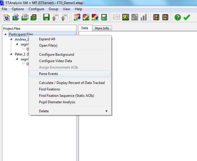
27 6 Parsing Events 6.1 Definition of Events When data is recorded from an eye tracker that records.eyd type files (Argus ETServer, or ASL ET5, 6, or7), or.ehd type files recorded with the ET3Space (or ASL EyeHead Integration) feature, recording can be started and paused multiple times on a single data file. Continuous data, between a start and pause, is referred to as a data segment. An eyd or ehd data file can, therefore, have multiple data segments. (ETMobile or ASL MobileEye csv type files always have only a single data segment.) When a data file is opened in ETAnalysis, the tree diagram at the left of the main window shows the file name and also shows all of the data segments on that file as sub nodes under the file name. ETAnalysis can further divide each data segment into to sub-segments based on various conditions involving time, XDAT values or mark flags. These sub-segments are called Events and the process is called Event Parsing. All subsequent processing, such as finding fixations, etc., is done on the basis of Events. An entire data segment may be an event, a single sub-section of the segment may be an event, or each data segment may be split into multiple events. Initially, the tree diagram shows one event, labeled Default Event, as a sub-node to each segment. The Default Event is the entire segment. The command to parse events is available from the context menu as shown below. The context menu is invoked by right clicking either the file name or an individual segment on the tree diagram. (If invoked by right clicking the file name, it will apply to all segments in the file; if invoked by right clicking a segment, it will apply only to that segment). If Delete(Delete Events is selected from this menu, or if event parsing fails, the segments under the selected node will revert to the Default Event. 27

28 28

29 The user is then presented with the Configure Events dialog shown below Selections on the dialog will be explained in the following sections. 6.2 Event Start condition The start condition can be one of the following: None. The event starts immediately with the first data record in the segment. XDAT. The event starts on the first record that has an XDAT value contained in the user-defined list of Start values; or, if the user has set the radio button to Any change in value, on the first record with an XDAT value different from the previous record. Note: the XDAT value on the very first field is 29

30 always considered a change and will trigger an event if Any change has been selected. On the example below, events are set to start when XDAT changes to 1 and when XDAT changes to 2, or to 3. Mark_Flag. The same as XDAT, except that the event starts on the first record that contains one of the specified Mark Flags. If Any change radio button is set, the event will start on the first record containing any mark flag. Time. The event starts at the specified time, entered as number of seconds from the beginning of the segment. The user can specify more than one start time value to create several events. In the example shown below, the first event would start 10.5 seconds after the beginning of the data segment, the next event would start 20 seconds after the beginning of the segment, and third event would start 30 seconds after the beginning of the segment. It is important to note that this can create overlapping events, if one event specifies an end time that is later than the start time for a subsequent event. If you create multiple events by start time, pay careful attention to the stop condition (described in the next section). Skip seconds before start. If Start Trigger is None, XDAT or Mark_Flag, user can also specify additional interval that will be skipped before the event start. In other words, if the skip time is t, the event will start t seconds after the Start Trigger is encountered. Suppose, for example, that the Start Trigger is XDAT, and that any change in value and Skip 5 seconds are specified. Further suppose that the first change in XDAT is 7 seconds from the start of the segment. In this case the first event will start 7+5=12 seconds from the beginning of the data segment. 6.3 Event Stop condition Event stop (or end) conditions are very similar to start conditions and contain the same choices, plus one additional choice called Next Event Start. The Start and Stop Triggers can be different. Almost any combination of Start and Stop conditions can be used. The dialog grays out the combinations that are illegal. Next Event Start means that there is no explicit stop condition, and the event will end when the next Start condition is encountered. 30

31 Note that when the stop condition is a time value, it specifies event duration rather than a time from the beginning of the segment. This is different from the time start condition, which is time from the segment beginning. Special cases: 1. In most cases the event continues until the stop condition is met, and any start conditions are ignored until the event has ended. One exception is when the stop condition is Next Event Start. The other exception is when the start condition is a time value. In this case, an event can start before the previous event end, and overlapping events are possible. 2. If the stop condition is never satisfied, the event continues to the end of the data segment. 3. If the Stop Trigger is None, the event continues to the end of the data segment. 4. If the Stop Trigger is Time, the value determines the event duration. In other words, stop time is measured from the event start rather than from the segment start. 5. If multiple XDAT or Mark_Flag values are specified as Start Triggers and the Stop Trigger is Time, then a different duration may be specified for each Start Trigger. In the example shown below, all events starting with XDAT=1 will continue for 10 sec, events starting with XDAT=2 will continue for 20 sec and events starting with XDAT=3 will continue for 30 sec. 6. If Start Trigger is XDAT or Mark_Flag and Stop Trigger is Time, the next event will start only after XDAT / Mark_Flag has changed. For example suppose that the Start Triggers are XDAT values 1 and 2 and Stop Triggers are Duration values 10 and 15 seconds. Further suppose that the first 20 sec in data segment have XDAT=1, the next 20 sec have XDAT=0, followed by 20 sec with XDAT=2. The first event will start with the first record of the data segment ( XDAT = 1) and will end after 10 seconds. The remaining 10 sec of data with XDAT=1 will be ignored. The next event will start 20 seconds from the beginning of the segment, on the first record containing XDAT=2, and will continue for 15 sec. 6.4 Parse by Video If there are no markers saved within the data file to aid in parsing data based on task or stimulus, it is possible to visually parse the data using the eye tracker scene video, if a video is available. This possibility is available if project is type ETMobile (csv data files); or if the project Stimulus Type is Videos or Both, and the scene video has been properly configured as described in section

32 To use the Parse by Video featue, Click Show Video in Configure Events window (B), then select the start and end frames of each stimulus presentation or task (C). Use the Play button or the video slider to advance to the vicinity of the desired start or stop frame. Once in the vicinity of the frame you want to select, use the left and right arrow keys or frame advance buttons to conveniently find the proper frame. When done marking start and stop frames, close the video player and choose Ok in the Configure Events window. A B C 6.5 Additional options Zero time origin. By default, Zero time origin is selected and the time stamp of the first record of each event will be reset to zero. The time of each record in the event is calculated with respect to the first record of the event. To make each event record show a time stamp corresponding to time from the beginning of the data segment, uncheck this box. Stop after first event. If this option is selected there will be not more than one event in the segment. After the end of the first event, the program will not start another event in the data segment. Discard incomplete events. Do not create an event if stop condition is not met before the end of the segment. For example if an event stop condition is XDAT = 2, and after the event begins no record with XDAT=2 is encountered before the segment end, this event will not be created. If Discard incomplete events is not checked, this event will be created and will end at the end of the data segment. 32

33 Continue events with same duration. Available only when both Start and Stop triggers set to Time. When this option is selected, program will continue parsing events with the same duration as the last defined event until the end of the segment is reached. Use as a project default. Use the current Configure Event dialog selections as the default for future event parsing operations. 33

34 7 Configure Static Background Images Static backgrounds are applicable if static background images have been presented to participants in ETServer, ET3Space, or Stimulus Tracking projects. This type of analysis will be most appropriate when subjects looked at static images such as pictures, text, web page images, etc. If subjects looked at dynamic presentations, or if gaze was recorded with respect to a head mounted scene camera image, analysis with respect to moving images may be more appropriate, and this is discussed in a subsequent section. In order to display 2-dimensional plots or heat maps it is necessary to configure one or more Backgrounds. A Background may be a blank screen, drawing or image that represents the scene viewed by the subject. If an image file is used, it can contain an image that was displayed on the presentation computer, a digital photograph of the scene (typical for head mounted optics), or a drawing that represents the scene that was viewed by the subject (for example, a sketch of an instrument panel that the subject viewed). If the image is a drawing of a physical scene that was viewed by the subject (I.e., an instrument panel), it should be to scale so that features in the drawing have the same spatial relation to each other as the real features. If the image is a photograph of the a physical scene that was viewed by the subject, the photograph should be taken straight-on to avoid perspective distortion. The program supports the following file formats: BMP, JPEG (JPG), GIF, or PNG. In order to superimpose point of gaze on the image, the program needs to know how to translate the eye tracker coordinates to the pixel location on the image (called VGA coordinates). To define the transform we need to specify two points with known image locations and eye tracker coordinates. These are called Attachment Points. It is best if the attachment points have widely separated vertical and horizontal coordinates, ideally near two opposite corners of the image. These points should be easily identifiable landmarks in the image. The eye tracker coordinates corresponding to the attachment points on an image file can be determined in advance. If table mounted eye tracker optics were used, display the image just as it was displayed to the subject, and use the Calibration Points Configuration dialog (ETSever or ASL ET7) or Set Target Points function (ASL ET6) to find the scene camera pixel coordinates associated with any point in the scene image. See the Eye Tracker manual for details. If ET3Space (or ASL EyeHead Integration) was used, use the pointer test function, or measure to find the ET3Space coordinates associated with any point in the scene image. See ET3Space (or ASL EyeHead Integration) manual for details. Any background that has been configured and made part of the project can be designated the default background. If other image files have the same resolution and will have the same correspondence between image and eye tracker coordinates, the default background attachment points can be used for these image files as well without requiring the attachment point placement procedure for each file. From the ETAnalysis main menu, select Configure Background Image(s) 34

35 A tab labeled Configure Backgrounds will appear in the right pane of the ETAnalysis program window. From the upper left corner of the Configure Backgrounds tab, left click the pull down menu labeled Background and select Create Single Background. or click the Add New Background button. A Create Background dialog will appear. 35

36 In the Configure Backgrounds dialog, click the Add New Background button A Select New Background Image dialog will appear. Blank Background Image If plots are to be superimposed on a blank screen, set the radio button to Use Blank Background Image and select the color and size of the desired image. Type any text in the Background Name box. This name will subsequently identify this image and associated configuration parameters. Under Eye Tracker coordinates select the horizontal and vertical gaze coordinate values that will correspond to the top left and bottom right corners of the blank image. For csv and eyd data, top left coordinates of (h = 0, v = 0) will usually be appropriate. Appropriate bottom right coordinates will usually be (h=640, v=480) for csv file (made with ETMobile or Mobile Eye systems) and eyd files made with ETServer or ET7 systems. For eyd files made with ET6 systems, bottom right coordinates of (h = 260, v = 240) will usually be appropriate. If using ET3Space (ehd files), the logical coordinate space depends on the physical size of the scene plane. 36

37 When the OK button is clicked, a blank image will appear with attachment points, corresponding to the top left and bottom right eye tracker coordinates, labeled P1 and P2 at the top left and bottom right corners. Click the Save & Close to close the image window. This background image with attachment points is now part of the project, and will be available for superimposing scan plots and heat maps. Create Background Image From File If an image file (rather than a blank screed) is to be used, set the radio button to Create Background from image file, click the browse button under Image File, browse to the desired jpg, bmp, gif, or png file. If the project already has a default background with attachment points that will be correct for the new image as well, check the box labeled Copy attachment points from default background. Attachment points are explained in more detail in the next section. Type in a Background Name, and click OK. The image from the selected file will appear. If Copy attachment points from default background was checked, the two attachment points will be shown. Just click Save & Close to add the configured background image to the project. If Copy attachment points from default background was not selected an Add/Edit Attachment Points dialog will automatically appear. (If Copy attachment points from default background was selected by mistake, click Attachment Points (Add/Edit Attachment Points to bring up the dialog.) Select two easily identifiable landmarks near opposite corners of the image, as previously discussed, and type in the Eyetracker Coordinates for each of these points. Enter the coordinates for one of these points in the Point 1 column (usually a point near top left), and the coordinates for the other in the Point 2 column (usually a point near bottom right). In the example, below, the eye tracker coordinates were previously determined to be (65,55) and (575,362), respectively. With radio button set to Point 1, use the mouse to click on the corresponding point in the image. A red dot with the label P1 should appear at that point, and the VGA coordinates of the point will appear in the VGA Coordinates section. With the radio button set to Point 2 (it should 37

38 automatically move there when point 1 is entered), click on point 2 in the image. A red dot with the label P2 will appear at that point, and the VGA coordinates will be entered. Ignore the Scene Plane no unless the image is to be used with ET3Space (.ehd) type data. If the background is an image file that was viewed by the subject, and if the corners of the image area were visible on the subject display, then two of the image corners can be used as the landmarks for attachment points, as shown in the example image below. 38

39 Click OK to close the Add/Edit Attachment Points dialog. Open and configure as many images as desired for use in the project. Be sure to give each a unique Background Name. If multiple image files have the same resolution and were displayed to the subject in the same way, then it will not be necessary to find unique attachment points for each of them. Set attachment points on one of the set, as described above, and use that image as a default for attachment points on the others. This is described in more detail below, in section Setting attachment points on the calibration target point display image The calibration target point display is a special case. *.eyd type data files contain the calibration target point coordinates used for the last calibration before the file was opened. The coordinates of target points 1 (upper left) and 9 (lower right) can be automatically extracted from the file and entered as attachment point Eye tracker coordinates. Select an image of the target point display as the Image File on the Select New Background Image dialog. Use the drop down menu on the Add/Edit Attachment Points dialog to select a data file that is part of the current project, and click the Set from target points 1 and 9 button. Then click on the image of points 1 and 9 to set the attachment points. If dealing with ET3Space (ehd) data, the scene plane must also be specified, and if not the calibration surface (scene plane 0), the program will offer to use points C and A instead of calibration targets 1 and 9. Points C and A are two of the points (in this case upper left and lower right) used to specify all 39

40 scene planes. See the ET3Space (or ASL EyeHead Integration) manual for further explanation of these plane definition points. 7.2 Using a default background image If two image files have the same resolution and are displayed the same way (by the same computer application, etc.) then a given image pixel, say the 20 th pixel from the left on the 20 th row, will appear in the same spot on the monitor screen for both images when displayed to the subject. This pixel will therefore correspond to the same gaze coordinate for both images. The same information can used to transform between gaze coordinates and image coordinates for both images. Assume that Image_1.jpg, Image_2.jpg, Image_3.jpg, and Image_4.jpg were all created the same way and were displayed to the subject the same way. Add Image_1.jpg to the project, give it a name, for example Image1, and set attachment points as previously described. On the Configure Background Selection window, set Default Background (at the top of the window) to Image1. Now open the Create Background dialog, browse to Image_2.jpg, name it, check the box labeled Copy Attachment Points from Default Background, and click OK. Image2 should appear with red dots labeled P1 and P2. They will be in the same position as they were on Image1, but since it is a different image they will probably not be on easily distinguished landmarks in the image. That is OK. The transformation between gaze and image coordinates will be correct. Leave Image1 as the default background and repeat the procedure for the other two image files. 7.3 Images to be used with ET3Space data Gaze data collected with the ET3Space (or ASL EyeHead integration) feature can be on different scene surfaces. Every data sample contains a scene plane number, and a set of coordinates that represent gaze position on a reference frame attached to that surface. The gaze coordinates represent real distance units (inches or centimeters) along two coordinate axes that have an origin and orientation on the surface specified by the user (see ET3Space manual). A background image to be used with ET3Space data may depict multiple scene planes, and separate attachment points must be defined for each. It is important that each scene plane surface is depicted without significant perspective distortion. For example a straight on photo might be taken of each surface and assembled into a single image with a picture editor. Alternately a graphics or drawing program may be used to create proportionately correct depictions of each surface. Each surface depicted must have two landmarks, preferably near opposite corners of the surface, whose gaze coordinates are known. These will be used as attachment points. The gaze coordinates can be determined by measuring along the user defined coordinate axes on a given surface, or by using the eye tracker Pointer Test mode. Open the image file in ETAnalysis as previously described. On the Add/Edit Attachment Points dialog, set the Scene Plane to 0 (at the bottom of the dialog window), and enter the gaze coordinates for the scene plane 0 attachment points under Eye Tracker coordinates. Click on each of the plane 0 attachment points on the image, and dots labeled P1 and P2 will appear as previously described. 40

41 Now change the Scene Plane to 1. Enter the gaze coordinates for the plane 1 attachment points under Eye Tracker coordinates. With the radio button on P1, use the mouse to click the first attachment point on the depiction of scene plane 1. Set the radio button to P2 and click the second landmark on scene plane 2. The labels on these points will appear as P1,1 (plane 1, point1) and P1,2 (plane1, point2). The labels on the plane 0 attachment points will change to P0,1 and P0,2. Repeat the procedure for any other scene planes depicted. 7.4 Exporting and Importing Background configurations Background configuration information can be exported to an XML type file, for future import to other projects, or to protect against accidental loss. On the Configure Backgrounds tab, pull down the Background menu and select Export. Browse to the desired folder location, type in a file name and click Save. Background configuration information for all current backgrounds (all those listed under the Current Background: pull down menu on the Configure Backgrounds tab) will be saved to the specified file. To import a set of configured backgrounds that was previously saved (exported), first open a Configure Backgrounds tab if not already opened (Configure Background Image(s) ). Left click the pull down menu labeled Background, and select Import. Browse to the previously saved xml file and click Open. All backgrounds in the saved set will now be available under the Current Background: pull down menu. Note that the saved xml file contains the scaling information for the set of backgrounds, created as described in the preceding sections, and has pointers to the original image files. It does not include the actual image files. For the import to work, the original image files must be at the same path location as when the xml file was created. If one of the image files is no longer in the same location, when that file is selected, on the Current Background: pull down menu, a warning message like the one shown below will appear. The message shows the path and name of the file that could not be found. To restore the configured background image, click Yes to bring up a browser window, and browse to the current location of the image file. To import configured backgrounds to an ETAnalysis project on another PC, the saved xml file, and all of the image files must be copied to that PC. Unless the image files are copied to the same path locations as on the original PC, it will be necessary to browse to each image file as described above. 41

42 8 Static Areas of Interest Areas of interest (AOIs) are rectangular subsections of the scene surface defined by the user. In the case of ET3Space (ehd) data there are multiple scene plane surfaces and areas of interest can be specified on each of them. Many of the statistics that can be produced by ETAnalysis relate fixations to AOIs. AOIs are defined by top, bottom, left, and right boundaries, expressed in the scene reference frame. If the project has a background image corresponding to the scene, AOIs can be defined graphically on the background image. This is usually the easiest method. Alternately the boundaries can be entered manually (typed in). In this case the boundary coordinates can be determined using the Eye Tracker Set Target Points function; or in the case of Eye Head Integration data, by measuring or using the Eye Tracker Pointer Test function. Each AOI can be given a name and collections of AOIs are organized in named sets. The project can contain multiple sets of AOIs. An event can be associated with any AOI set in the project for the purpose of computing fixation and dwell statistics. AOI sets do not appear in the tree diagram, but all sets currently available to the project are listed in a drop down menu on the Configure Areas of Interest dialog and all other dialogs on which an AOI set must be specified. 8.1 Defining Areas of Interest graphically From ETAnalysis main menu select Configure Areas of Interest (static, graphically) 42

43 In the AOI Configuration dialog select a Background image and in the AOI Set selection combo box enter a name for the AOI set by typing it in the combo box. If this is the first set created in the project, the default name will be Aoi_Set_01. This name can be changed at any time. From the AOI menu, select Draw Area of Interest (or use the shortcut <Ctrl>A). The mouse pointer will change to an AOI symbol, and remain in that form until the right mouse button is clicked Draw rectangular areas To draw a rectangular AOI click to depress the "Draw rectangular AOI" button. Holding down the left-mouse button, drag a rectangle of any desired size and release the mouse button when done. The area will appear as a shaded rectangle (drawn over the left penguin head, in the example below), and an AOI Properties window will appear. Replace the default name ( AOI 1 in the example below ) if desired, by typing over the default name. If using Eye Head Integration data (ehd file), set the Scene Plane: to the scene plane number on which the AOI has been drawn. If not ehd data, leave the Scene Plane set to 0. The line thickness and color of the area outline will default to the values shown, and can changed if desired. Click the OK button on the AOI Properties window. The AOI Properties window will close, and the AOI will be shown by a an outline of the specified color, with corner and side handles (small white squares) as shown below. A legend box at the upper right of the pane lists all areas currently created. 43

44 When the mouse arrow is hovered over one of the handles, it will change to a double arrow symbol and the AOI can be stretched or compressed in the indicated directions by holding down the left mouse button and dragging. When the mouse arrow is held inside the area, it becomes a hand symbol and the entire area can be moved by dragging with the left mouse button. Right clicking with the area pops up a menu that can be used to bring back the AOI Properties dialog, make a copy of the area, or delete the AOI. 44

45 8.1.2 Draw Polygons To draw a polygon, first click to depress the draw polygon button. Left click on the image open an AOI Properties dialog and set the AOI name and other properties just as with rectangular AOIs. Note, however, that no AOI is draw until the AOI Properties dialog is closed by clicking OK. At this point a triangle will appear at the spot on the image that was left clicked. The triangle (just above the middle penguin head in the example, below) will have a handle at each vertex. Left drag any of the handles (mouse arrow changes crossed arrows when on a handle) to move just that vertex, or place the mouse inside the object (mouse arrow changes to hand) and left drag the entire object. Left clicking inside the object will also cause a bounding box, formed with dashed lines to appear on the object. Left click on the bounding box to make it disappear. Click on one of the lines to add a vertex (mouse arrow changes to gray cross when held in proper position to form a new vertex), and, holding down the left-mouse button, drag the newly created vertex to the desired position; repeat this process until all sides of the polygon are constructed. See the example sequence below. 45

46 Continue in a similar fashion to obtain the result shown below. As with rectangular AOIs, right clicking with the area pops up a menu that can be used to bring back the AOI Properties dialog, make a copy of the area, or delete the AOI. 46

47 8.1.3 Saving AOI sets and other dialog window features To create a new AOI as part of the current AOI set, simply depress either the rectangle or polygon button, and left click on the image beyond the boundary of any existing AOI. Then proceed as described in the previous sections. Important: if are using multiple scene planes (typical for head mounted optics with ET3Space or EyeHead Integration feature) be sure to select the appropriate scene plane in the AOI Properties dialog. To make a new AOI set, select Areas of Interest(Create Blank AOI Set, then proceed as described in the previous sections. To edit a different AOI set, previously created in the project, use the AOI Set: and Background: drop down menus to select the desired AOI set and background image. Selections in the Areas of Interest drop down menu can be used to delete all of the AOIs in a given set, or to delete the entire set. To make a new AOI set by modifying an existing set, select Areas of Interest Copy AOI Set. The currently selected AOI set will be copied as a new set and can be named and modified as desired. AOI sets can be saved for export to other projects, and AOI sets that have been saved by other projects can be imported to the current project. To save the current AOI sets for potential export to other projects, select Areas of Interest Export AOI sets to File. Use the resulting browser window to specify a path and file name for the AOI sets. All current AOI sets will be saved in the form of an XML file. To import a AOI sets saved in other projects, select Areas of Interest Import AOI sets from File, and browse to the previously saved XML file. The AOI sets on the file will be imported and will replace any AOI sets already in the current project. Be sure to record the names and locations of these files or use names and locations that will be remembered. A set of buttons at the top of the Configure AOIs Graphically window can be used to adjust image zoom setting, lock or unlock the window for further modifications of AOI modification, edit the attachment points (see section 7.1), and save an image file of the current window in bmp, jpg, tiff, or png format. Hover the mouse over each button to see its function. AOIs created graphically can be edited manually, as described in the next section. AOIs created manually, will be displayed on the Configure AOIs Graphically window when the appropriate AOI set is selected, and can be edited graphically When finished creating and exporting AOI sets, click the Save & Close button at the upper right of the Configure AOIs Graphically window to save the contained AOI sets as part of the current project. 47

48 8.2 Defining Areas of Interest manually To create AOIs manually, select Configure Areas of Interest (static, manually) from the ETAnalysis main menu. A table entry dialog will appear as shown below. To create or edit AOIs manually, select Configure(Areas of Interest (manually) from the ETAnalysis main menu bar. A table entry dialog will appear as shown below. Select the Edit Rectangles tab for rectangular AOIs or the Edit Polygons tab for multi-sided AOIs. The View All tab shows coordinates for both rectangular and multi-sided AOIs, but this tab is only for viewing the coordinate values and cannot be used for editing. Manual AOI creation or editing is usually done with rectangular areas. In this case, the left, right, top, and bottom boundary coordinates are specified. In the case of polygon AOIs, each horizontal and vertical vertex coordinate are specified. VnX is the horizontal coordinate for vertex n, and VnY is the vertical coordinate. If creating a new polygon AOI, only 6 vertices are available. Polygons with more than 6 sides, must be created graphically. However, if polygon with over 6 sides has been created graphically, all the vertices will listed and can be edited manually. If creating a new AOI set, click the Command button and select Create Blank Aoi set. Next to Selected AOI Set type in the desired name for the AOI set. In the appropriate columns type the AOI name, and boundary coordinates or vertex coordinates. The boundary or vertex coordinates are floating point values. If the AOI set will be used for ET3Space (ehd) data, be sure to include the scene plane number. The scene plane number must be an integer. As soon as an entry is made on one row, another row becomes available for new entry. To delete an AOI, highlight the row and select Delete Selected AOIs from the Command drop down menu. To edit an existing AOI set, select the set from the Selected AOI Set drop down menu. To close the dialog and save the current AOI sets click Save & Close. To close the dialog without saving any changes made (since the dialog was opened), click the X in the red square next to the tab label. Argus and ASL Eye Tracker gaze values have horizontal coordinates that increase as gaze moves to the right, and vertical coordinates that increase as gaze moves down. For rectangular areas therefore, on any given row, left boundary values must be less than right boundary values and top values must be less than bottom values. In the case of ET3space (and ASL EyeHead Integration) scene planes there may be occasionally be a scene plane for which it is not immediately obvious what is meant by horizontal and what is meant by vertical. Horizontal always refers to the y axis and vertical to the z axis on ET3Space scene planes. See the ET3Space manual (or ASL EyeHead Integration manual) for a more detailed explanation of scene plane coordinate frames. 48

49 9 Event Correspondence with Background images and AOI sets Once Backgrounds and static AOI sets have been defined, each event in the project can be matched with a particular background and AOI set. These correspondences are specified on a AOI Sets and/or Background Correspondences dialog. The dialog is available as a selection under the Configure Menu, and also automatically appears when a Fixation Sequence computation is requested as described in the next section. An AOI set can be explicitly assigned to each event, segment, or file. Alternately, the first XDAT value in each event can be used to specify the AOI set. In the example above, event 1, from any file and segment in the project, is assigned the Penguin background image and PenguinAOI AOI set. Event 2, from any file and segment in the project, is assigned the Koala background image and KoalaAOI AOI set. The blank background and aoi set are not assigned to any event. The AOI Sets and/or Background Correspondences dialog defines the rules for selecting the background and AOI set that will be used with each event for calculating fixation sequence results. An empty field means ANY. If an XDAT value is specified, it will be the value of XDAT in the first data record of the event. If no rule is satisfied a default assignment will be used. 49

50 There is an implicit logical AND between fields. For example, if both an XDAT value and an event number are specified on one row of the dialog, the AOI set specified on that row will be used only if that event number also has the specified XDAT value in its first field. Otherwise, a default assignment will be used. If there is only background and set of AOIs, just leave all fields blank. Note that each Background and AOI set defined in the project must appear on the dialog, even if they will not correspond to any event. In the example below, the any event with an initial XDAT value of 1 will be associated with Penguins background and AOI set; while any event with an initial XDAT values of 2 will be associated with the Koala background and AOI set. In the following example, Penguins will be associated with event 1 on the Andrea_1.eyd file, but with event 2 on the Peter_1.eyd file, etc. 50

51 10 Fixation analysis During normal scanning of a visual scene, eye movement is characterized by a series of stops and very rapid jumps between stopping points. The stops, usually lasting more than 100 ms, are called fixations, and it is during these fixations that most visual information is acquired and processed. These rapid jumps between fixation points are called saccades. Saccades are conjugate eye movements (both eyes move together) that can range from 1 to 50 degrees of visual angle, and achieve velocities as high as degrees per second. Very little visual information is acquired during saccades, primarily because of the very fast motion of the images across the retina, and an associated elevated visual threshold by the brain, just prior to and during a saccade, called visual image suppression. The eyes are not completely stationary during fixations, but exhibit a variety of small involuntary motions, usually of less than one degree visual angle, called flicks (or micro saccades), drift, and tremor. The eyes can smoothly track targets that are moving no more than about 30 deg/sec (faster for some people). These conjugate, slow tracking eye movements are usually called smooth pursuit and act to partially stabilize slowly moving targets on the retina. Similar slow conjugate eye movements called compensatory eye movements partially stabilize the visual field during either active or passive head or trunk motions. When gaze data is analyzed, a common practice is to first reduce the data to a set of fixations, since in most cases these are the periods when visual information was stable on the retina and available to be processed by the brain. The following subsections describe the algorithm used by ETAnalysis to compute periods of fixation. Video base eye trackers measure line of gaze with respect to the eye camera optics. In the case of systems with table mounted the data report gaze with respect to a stationary display surface (usually a display monitor located just above the eye camera optics). When the fixation algorithm is applied to this data, it finds periods of relatively stable gaze with respect to the stationary display. Note that sometimes, if the subject s head is moving, these periods of stable gaze may be produced by compensatory eye movements. However, the fixation algorithm does not make these distinctions. It just finds periods of stable gaze measurement. ET3Space (ehd) data (produced by an eye tracker with head mounted optics and an independent head tracking device) also specifies point of gaze on stationary surfaces, and when the fixation algorithm is applied to this data the situation is the same as that described in the previous paragraph. In the case of head mounted optics used with a head tracker and just a head mounted scene camera (not using ET3Space or EyeHead Integration feature) the gaze measurement is with respect to the subject s head (more specifically, with respect to the field of view of the head mounted scene camera). The fixation algorithm, when applied to this data finds periods of relatively stable line of gaze with respect to the head. Note that periods during which smooth pursuit or compensatory eye movements may be stabilizing gaze on some external target may not constitute periods of stable gaze data, since, during these periods, the eye is rotating with respect to the subject s head. 51

52 In all cases described above, fixations are computed with respect to the scene image frame of reference, which may either be a stationary surface (table mounted optics or ET3Space) or a head mounted scene camera image. Furthermore, in all of these cases, fixations can be computed using just the gaze data produced by the eye tracker. Areas of Interest on the scene do not need to be specified in order for fixations to be computed. Fixations computed in this way therefore appear as Fixation Nodes that are directly under an event node on the project tree diagram. This is the case addressed by the procedures described under the current section (section 10) of this manual. As described later in this manual, ETAnalysis is also able to define moving areas of interest which follow targets that move either with respect to a stationary display surface or with respect to a head mounted scene camera field of view. If moving areas of interest (MAOIs) are defined, then fixations may also be computed as periods during which the gaze remains relatively stable with respect to the boundaries of these areas. This may include periods during which smooth pursuit or compensatory eye movements stabilize gaze on a moving target. Note, however, that fixations defined in this way can only be computed if moving areas of interest have been defined, and can be detected only when gaze is within one of these areas. Such fixations appear as Fixation Nodes under Moving Area of Interest Nodes, and this type of analysis is discussed under section 16 of this manual. The same basic fixation algorithm, which is really an adjustable nonlinear filter, is used in all cases Origin of fixation algorithm The fixation algorithm used in ETAnalysis derives from work done by Lambert, Monty, and Hall, (1974), further developed by Flagg (1977) and Karsh and Breitenbach (1983), and others over the years. The method falls in the category that Duchowski (2003) labels dwell-time fixation detection as opposed to velocity-based saccade detection. The original rational for a minimum fixation duration was that the latency in beginning a saccade to a new target that was probably a measure of the minimum time needed by the nervous system to process visual information meaningfully, and therefore the shortest sensible snapshot. The shortest latencies were reported to be about 100ms, with latencies ranging up to about 300 ms (Alpern, 1969; Young, 1970, Yarbus, 1967). Looking at more recent data, saccadic latencies seem rarely to be less than 150 ms under most conditions, and are more typically over 200 ms, but express saccades can have latencies as short as 90 to 120 ms when the old fixation target disappear before the new target appears, or if the new targets are predictable (for example, see Darrien et.al. 2001, Fischer and Ramsperger, 1984). The default minimum in the ETAnalysis fixation program is 100 ms. Note that if the data is collected at 60 fields per second, it corresponds to 7 samples. The 1-degree minimum change in gaze position required to define a new fixation is based, loosely, on the fact that miniature eye movements (tremor, drift, and micro-saccades) are generally smaller than 1 degree. Of course they are often significantly smaller than 1 degree, and the minimum could arguably be smaller. It is important to take into account the quality of the measurement. No matter what the underlying physiology, it is only possible to detect changes in fixation position that are larger than the measurement noise. There is no firm definition for a fixation. It is less a physiological quantity than a method for categorizing sections of a data stream. Sensible selection of criteria depends on the experimental goal 52

53 and the characteristics of the measurement a well as underlying physiology. There are quite a few different algorithms in the literature for detecting fixations, all of which represent logical strategies. Processing the same data with different algorithms or different parameters for a given algorithm, all of which may be justifiable, can easily result in a different number of fixations and different set of fixation start and stop times, and positions. This makes it important to report the method used. The default parameters in the ETAnalysis fixation program are chosen with the hope that they will at least be reasonable in the majority of cases, but they were not intended to promote a particular definition for a fixation. The program is really an adjustable non-linear filter. It is useful to look at horizontal and vertical position time plots for some sections of data, and to superimpose the fixation start and stop points determined by the fixation program for that section of data. The researcher can verify that the program is doing a reasonable job of choosing periods that the researcher would regard as fixations, or adjust the algorithm parameters as necessary. References: Alpern, M. Types of Movement, H. Davson (Ed.) The Eye (vol.3, 2nd ed), Academic Press, New York, Young, L., Recording eye position, M. Clynes & M. Milsum (Eds. ), Biomedical Engineering Systems, McGraw Hill, New York, Yarbus, A.L., Eye Movements and Vision, Plenum Press, New York, A.T. Duchowski, Eye Tracking Methodology Theory and Practice, Springer-Verlag, London, Darrien, Herd, Starling, Rosenberg, and Morrison, An analysis of the dependence of saccadic latency on target position and target characteristics in human subjects, BMC Neuroscience 2001, 2:13 Fischer B, Ramsperger E: Human express saccades: extremely short reaction times of goal directed movements. Exp Brain Res 1984, 57:191-: Fixation Algorithm Description The fixation algorithm relies on three Criteria. The first is used to determine when a fixation starts; the second is used to determine whether subsequent data samples are part of the same fixation; and the third is used to determine which data samples should be averaged together to determine the final fixation coordinates. To "start a fixation" the program looks for a specified period (Minimum Fixation Duration) during which gaze has a 95% confidence interval (twice the standard deviation) of no more than a specified amount (Threshold 1 value). The average horizontal and average vertical gaze position during this period is the temporary fixation position. To end the fixation, it looks for a specified number of sequential gaze position samples to be farther than a specified distance (Threshold 2) from the temporary fixation position. The final fixation position is the average position of all data samples between the beginning and end of the fixation. The exception is that any gaze coordinates that were farther than a specified value (Threshold 3) from the initial fixation position are not included in the average. 53

54 The reason that more than one sample must exceed threshold 2 in order to end a fixation is so that an extraneous spike in the data will not cause the fixation to end. The reason for Threshold 3, is to exclude such spikes from being included in the fixation position computation. If a fixation has started and pupil recognition is lost (for example, due to a blink) for less than the time specified as Maximum Pupil Loss, then this does not cause the fixation to end. The period of pupil loss is ignored, the gaze position on the first record for which the pupil is again recognized is compared to Threshold 2, and process continues as previously described. If pupil recognition is lost for a longer period, the fixation is considered to have ended at the beginning of the recognition loss period. The initial default value for Minimum Fixation Duration and Threshold 1 are is 100 msec and 1 degree visual angle, respectively. The default for Threshold 2 is also 1 degree, and the default number of samples that must exceed Threshold 2 to end a fixation is 3. The default for Threshold 3 is 1.5 degrees. The default for Maximum Pupil Loss is 200 msec (the maximum duration of most blinks). All of these parameters can be adjusted by the user. The user can set adjusted default values for the project and can also adjust these parameters individually for every fixation set created. When converting time periods to a number of samples, note that the period is the inter-sample period times one less than the number of samples. For example, the period between sample 1 and sample 7 is 6 sample periods. For a system operating at 60 Hz this is 100 msec. If data was collected with an eye tracker that used head mounted optics and the Argus ET3space (or ASL EyeHead Integration) feature, the data file will contains enough information for the program to calculate visual angles. In other cases the user must specify the number of eye tracker units per degree visual angle. 54

55 10.3 Setting Default Fixation Criteria To view or adjust the current default values for fixation parameters, select Fixations from the Configure menu on the main menu bar Begin Fixation Criteria A fixation is considered to start when the gaze data is sufficiently stable for a minimum time. More specifically, a fixation starts when a minimum number of sequential horizontal and vertical point- 55

56 of-gaze coordinate samples have a standard deviation below half of Threshold 1. The rational for specifying twice standard deviation as the threshold is that a normally distributed random variable will have about 95% of its values within the range of two standard deviations. The threshold value is expressed in units of degrees visual angle, and Threshold 1 has a default value of 1 degree. The minimum time (T1)is specified in seconds, and the program selects the number of samples that most closely corresponds to the specified time. The default value for T1 is 0.1 sec. Note that the time interval covered by n samples is the sample period multiplied by n-1. At a 60 Hz update rate, for examle, 0.1 sec corresponds to 7 samples. The user can change T1 and the program will recalculate the number of samples using the update rate that it reads from the file header. Once the program finds the minimum number of sequential sample points (corresponding to time period T1) that have a small enough standard deviation, the fixation is considered to start with the first of these data samples, and the average point of gaze value for this set of points is memorized as the fixation start position. Note that Time T1 is the minimum possible fixation duration End Fixation Criteria A fixation ends when several (default: three) sequential samples, as well as their average, deviate from the fixation start position by more than the Threshold 2 value (default: 1 degree visual angle). The deviation can be in either horizontal or vertical point of gaze coordinates. The data point preceding these samples is considered to be the last data sample in the fixation. Another reason to end the fixation is continuous loss of eye recognition for more than a specified time (default: 0.2 sec.). Shorter losses are assumed to be blinks and do not cause the fixation to end. The program uses the update rate to calculate the number of samples most closely corresponding to the specified time. The last selection on the End Fixation Criterion is the checkbox Treat CR loss as point of gaze loss. CR (cornea reflection) position is one of the features that the eye tracker uses, along with the pupil position, to calculate point of gaze. Some eye tracker configurations are able to make a less accurate estimate of gaze using only the pupil, while others always require the CR for valid data. The eye tracker Basic Configuration menu offers user a choice: use CR for low frequency correction, always use CR or never use CR (see eye tracker documentation for details). If the eye tracker is configured to never use CR, the checkbox should be unchecked. If CR is used for low frequency correction, the 56

57 selection is up to the user. If the eye tracker always uses the CR so should the file analysis program and the checkbox should be checked (that is the default). Note the eye tracker with desktop optics requires that the CR always be used (unless the subject s head is rigidly restrained), and in this case Treat CR loss as point of gaze loss should be checked Finding the final fixation position and excluding outliers The final fixation position is the average of all the points from the start point to the end point, but excluding some points considered to be outliers. Remember that a single point that is very far from the fixation start point doesn t necessarily end the fixation. There must be 3 (or some other specified number) in a row. This is so that a brief measurement noise spike will not end the fixation. The result is that there may be some far off points between the fixation start and end points that should be considered noise. Any points farther than Threshold 3 from the fixation start position will be excluded from computation of the final fixation position. Threshold 3 is specified separately for the horizontal and vertical axis, and the default is 1.5 degrees visual angle XDAT and Mark Flags Each fixation record shows the XDAT value that was recorded at the beginning of fixation. However, the XDAT value can change during the fixation period. If the user selects Show every XDAT value option, the program will create a line in the fixation list for every XDAT change as shown below: When the eye tracker is recording a file, the user can create marks on the data by pressing numeric keys on the keyboard. These flags can be displayed in the fixation list if user selects the option Show every Mark Flag. 57

58 By default these options are not selected Exact time For some fixation criteria, the user specifies a time interval in terms of seconds, and the program calculates the corresponding number of samples that comes closest to this time interval, based on the eye tracker update rate. The actual time interval is based on this number of samples and can be slightly different from the value that user requested. For example, if user defines maximum pupil loss as 0.18 sec and the update rate is 60 Hz, the program will use 12 samples, which correspond to an exact interval of sec. The Exact time group of items shows the exact time intervals based on the number of samples and exact update rate. This is information only Eye tracker units/degree (visual angle) If data was collected with an eye tracker that used head mounted optics and Argus ET3Space (or ASL EyeHead Integration) feature, the.ehd data file contains enough information for the program to calculate visual angles. In this case the Eye tracker units/degree box on the advanced Fixation Detection Criteria dialog can be ignored. If data was collected with an eye tracker using remote optics, the data will contain only point of gaze coordinates expressed in special eye tracker units. The visual angle represented by these units depends on the distance to the display, the size of the display, and the physical separation of the target points on the display, information not contained in the data. The user must specify a conversion factor to translate eye tracker units to degrees visual angle, and it must be specified for both the horizontal and vertical axes. For an Eye-Trac 6 system with table mounted optics (model D6), the scale factor values will typically be approximately 10. For an ETServer or Eye-Trac 7 with table mounted optics the values will typically be approximately 20. For ETMobile, Mobile Eye, or ETSever or EyeTrac7 head mounted systems, with the standard scene camera lens (and not using ET3Space feature), the scale factors will 58

59 usually be close to 10. For EyeTrac6 head mounted optics systems, with a standard scene camera and lens, the value will be approximately 5. Clicking the Calculate button brings up a dialog to help calculate these factors more precisely Visual angle calculator dialog Measure the distance from a subject s eye to the center of the scene display when the subject is in the most usual position. Enter the distance as Eye to scene distance. Any units of measure can be used, but all measurements must be made in the same units. Select two points on the scene display that are widely separated along the horizontal axis and two points widely separated along the vertical axis. Call the two horizontally separated points A and B, and the vertically separated points C and D. Use the Eye Tracker Set Target Point function to find the eye tracker coordinates of all four points. Be sure that A and B have the same (or almost the same) vertical coordinates and that C and D have almost the same horizontal coordinates. Use a ruler to measure the distance between A and B and between C and D. Enter the values in the boxes labeled Horizontal points A and B and Vertical Points C and D and click the Calculate button. The scale factors will appear in the boxes labeled Horizontal and Vertical. When the OK button is clicked on the Eye Tracker Units to Degrees window the computed scale factors are automatically entered in the Fixation Detection Criteria window. To close the Eye Tracker Units to Degrees window without entering the results in the Fixation Detection Criteria window, click Cancel. The Restore Defaults button will bring back the factory default values. 59

60 Detailed explanation of visual angle computations All fixation criteria are defined in degrees visual angle, i.e how much eye turns between measured points of gaze. Therefore we need to translate point of gaze data expressed in eye tracker units (remote optics) or real distance units on a surface (head-mounted optics with ET3Space feature) to degrees. If we assume that lines of gaze are more or less perpendicular to the surface (within about 20 degrees), visual angle A between two points is defined by the equation: tan(a) = D / S where D is the distance between the points, and S is the distance from the eye to the scene plane. In order to avoid time consuming calculation of tan -1 we use the fact that, for fixation analysis, we are only interested in small eye movements and we use the small angle approximation: where A is expressed in radians. tan (A) A There are 180/pi (= ) radians per degree. Combining the two equations and translating radians to degrees we get the equation that the analysis program uses to calculate visual angles: A * D / S where A is the visual angle in degrees, between two points separated by distance D, at a distance S from the eye. If data was collected with an eye tracker that used head mounted optics and Argus ET3Space (or ASL EyeHead Integration) feature, the.ehd data file will contain both the point of gaze coordinates (which allow us to calculate D) and distance from the eye to the point of gaze (S). In all other cases, the data will contain only point of gaze coordinates expressed in special eye tracker units. In those cases the analysis program takes the difference between point of gaze coordinates and divides by the user specified constant labeled Eye tracker units/degree. The precise value depends on distances and magnifications, which can vary. The user can change this value manually or use a built-in dialog to recalculate it, as described in the previous section Boundary Limits In some cases it may be obvious that any fixation positions beyond certain boundary limits must be artifacts. For example, in the case of an Eye-Trac 7 with desktop mounted optics (model D7), the scene space is usually a display screen with eye position coordinates of (0,0) in the upper left corner and (640,480) in the lower right. If the usual display screen size and component placement is used, the upper left and right corners of the screen will be near the range limits for proper corneal reflection detection. Correct gaze position may still be legitimately detected if the subject looks slightly beyond the edges of the screen, and gaze near the edges may sometimes be reported as just beyond the edges dues to measurement error. These conditions may result in gaze coordinates that are slightly less than 0, or slightly more than 640 horizontal or 480 vertical. However, any gaze coordinates that are far beyond these limits (for example, a horizontal gaze coordinate of 200) are probably artifacts due to 60

61 incorrect recognition of some image element as a pupil or corneal reflection, and probably not valid data. Usually, any such data will be extremely noisy and will rejected by the fixation algorithm, but the boundary limit feature can also be used to insure that no impossible gaze coordinate values will be considered fixations. To use boundary limits, click to check the Enable box, and click the Set/Check button to bring up the boundary limit dialog. Type in the desired boundary values. Those shown above are probably reasonable values for the typical model D7 example cited in the preceding paragraph. For a typical model D6 setup, more reasonable values might be negative 10 for the top and left, positive 270 for right, and positive 250 for bottom Creating Fixation sets Fixation sets are computed for data contained in Events and appear as nodes on the ETAnalysis tree diagram under the corresponding event node, with a name specified by the user. Each fixation set is created with a user defined set of parameters that define fixations. An event node can have more than one fixation set since the same data can be processed using different parameter values to define the fixations. Right clicking an event node, or any node above the event level on the tree diagram produces a context menu that includes a Find Fixations item. Selecting Find Fixations will bring up a Fixation Detection Criteria Dialog used to specify the parameters that will define a fixation. Clicking OK to close this dialog causes fixation sets to be computed for all events in sub-nodes under the selected node. For example selecting Find Fixations by right clicking an event node will create just one 61

62 fixation set using the data from that event. Right clicking the Data Files node and selecting Find Fixations will compute fixation sets for every event in the project, etc. A Basic Fixation Criteria dialog will open. Type a name for the fixation set (or leave the default name shown). The name can also be changed later directly from the node on tree diagram. If default parameters have already been set as described in the previous section, and if these parameters are the ones desired, simply click OK. Basic parameters can be changed, if desired directly on this dialog. Checking the Use as project default box, will make these changes the default for any subsequent fixation sets created, but previously created fixation sets will not be changed. To view or change all of the available parameters, click the Advanced Configuration button. This brings up the same dialog discussed in section Changes made to the defaults values will apply only to the fixation sets currently being created, unless the Use as project default box is checked, in which case these changes will become the default for any subsequent fixation sets created. Caution: One of the parameters not included on the basic dialog is the conversion from eye tracker units to degrees visual angle. In the case of head mounted systems with ETSpace (or ASL EyeHead Integration) feature, this value is computed automatically. In all other cases, be sure to read section , and implement the procedure to properly set the visual angle scale factor. These scale factors are set on the Advanced Configuration dialog Fixation data display Clicking OK on the Fixation Detection Criteria window will cause a new Fixation node to appear on the project tree diagram. When a fixation node is selected on the tree diagram, in the left panel of the main window, the data tab on the right panel displays a list of fixation points. 62

63 The table below explains the fields included for each fixation. All time intervals are shown in seconds Name Fix# StartTime Duration PupilLoss StopTime IntefixDur InterfixPupilLoss InterfixDegree ScenePlane HorzPos VertPos PupilDiam GazeLength StartField# StopField# CU_Field# XDAT MarkFlag Description Fixation number Time stamp of the first record in the fixation Difference between stop and start time Total time during fixation when point of gaze was not available Time stamp of the last record in the fixation Start time minus stop time of previous fixation (zero for first fixation) Total time between fixations when point of gaze was not available (zero for first fixation) Difference between this fixation and previous fixation in degrees visual angle (zero for first fixation). Calculation of InterfixDegree is explained below. Fixation scene plane number. ET3Space or EyeHead Integration only Average point of gaze horizontal coordinate during fixation Average point of gaze vertical coordinate during fixation Average pupil diameter during fixation Average eye to scene distance during fixation. ET3Space or EHI only video_field_# of the first record in the fixation video_field_# of the last record in the fixation CU_video_field_num of the first record in the fixation (optional, may be missing in the data file) XDAT value of the first record in the fixation. Note: If user selects Show every XDAT value option, the fixation list will include a line for each new XDAT value. These lines will be marked x in the firsts column to distinguish them from the fixation records. Optional column. If user selects Show every Mark flag option, the fixation list will include a line for each Mark value. These lines will be marked m in the firsts column to distinguish them from the fixation records The More Info Tab lists all of the information that was specified in the Fixation Detection Criteria window in order to create the fixation set, and also shows some summary information. The summary information items are: Event duration Number of fixations Average fixation duration 63

64 Average inter-fixation duration Average inter-fixation degree Frequency (fixations per sec) Pupil loss time o Before first fixation o After last fixation o Total within fixations o Total between fixations o Total loss for event Loss due to overtimes Event duration is the length of the data section defined as an event. This is the section of data over which the program tried to identify fixations. The first fixation may not have started until some time after the start of the event and the last fixation may have ended before the end of the event data. Average inter-fixation degree is the distance between fixations expressed in degrees visual angle. Pupil loss time is the time that a pupil was not recognized by the eye tracker. This includes blinks, lack of recognition due to poor discrimination, and loss of data fields as described below. Of course this cannot include periods during which the system thought it was recognizing a pupil, but was in fact mistakenly recognizing some artifact. The first 4 items under Pupil loss time should add up to the last item ( Total loss for event ). The eye tracker may occasionally lose one or more fields of data. This should be a rare occurrence, but the system detects this when it occurs and reports, as Loss due to overtimes, the number of fields lost multiplied by the field period. Other items in the summary list are self-explanatory. 64

65 11 Fixation Sequence analysis The Fixation Sequence Analysis compares a Fixations list to a set of Areas of Interest (AOIs). It reports the relation of each fixation to the defined AOIs, and computes related statistics. A similar analysis is done for Dwells, which are defined as sequential fixations that remain in the same AOI, and are discussed in section 12. This section discusses static Areas of Interest (sets of areas which retain constant shapes and positions for an entire event). It is also possible to define moving areas of interest, on a video showing a dynamic scene presentation. Working with scene video and defining moving areas of interest is discussed in section 16. To launch the fixation sequence and dwell computations right click any node in the tree diagram at the Fixation level or higher, and select Find Fixation Sequence (Static AOIs). The Fixation Sequence computation requested will apply to all sub-nodes under the selected node. An AOI Sets and/or Background Correspondences dialog will appear, and its use was previously described in section 9. When the OK button is clicked on this next dialog, the fixation and dwell sequence computations are performed and a fixation sequence node and dwell node are added to the project tree under each Fixation node selected as described above. The Dwell node is at the same level as the fixation sequence node, and is automatically created whenever fixation sequence computations are done. Dwell analysis is described in section 12. Fixation Sequence nodes and Dwell nodes always include sub-nodes with an AOI Summary table, a Transition table, a Conditional Probability table, and a Joint Probability table. Note: when parsing data into events (as described in section 6), be sure that a new event starts at every point in the data where the scene image changed and will be represented by a different AOI set Fixation Sequence Data list and Info tab Highlighting a Fixation sequence node on the project tree, in the main window left panel, displays a corresponding data list in the right panel. The Fixation Sequence List is the same as the Fixation list except that AOI number and name designations for each fixation are added. In each case the program has determined that the coordinates for that fixation are within the boundaries of the specified AOI. Fixations that are not inside any defined AOI are considered to be within AOI #0, named OUTSIDE (all defined AOIs are numbered starting with 1). 65

66 The More Info tab displays the rules used for selecting the AOI set (as described in the previous section), the AOI set selected, and a list of the areas and boundary coordinates that make up that AOI set. It also contains information about the first three AOIs viewed. The Fixation Sequence node on the project tree expands to show AOI summary, transition table, conditional probability table, and joint probability table sub-nodes AOI Summary Highlighting an AOI Summary node on the project tree displays an AOI summary table in the right pane of the main window. The AOI summary includes the following fields that are calculated for each AOI. All time intervals are given in seconds. Name AOI# AOIname ScenePlane FixCount %FixCount TotalFixDuration %TotalFixDuration AvgFixDuration AvgInterFixDuration AvgInterFixDegree AvgPupilDiam FirstFixTime XDAT Description AOI number. Zero represents the area outside all AOIs AOI name (from AOI properties) AOI scene plane; will be displayed only for EHD data files Number of fixations that were inside AOI Above value as a percentage of the total fixation count Total duration of the fixations inside AOI Above value as a percentage of the total duration of all fixations Average duration of a fixation inside the AOI Average time between the fixations that stayed inside the same AOI Average angle between the fixations that stayed inside the same AOI (in degrees) Average pupil diameter for the fixations inside the AOI. The average pupil diameter of each fixation is weighted with the fixation duration: AvgPupilDiam = SUM(fixation.avgPupilDiameter * fixation.duration) / SUM(fixation.duration) Start time of the first fixation inside AOI. If AOI contains no fixations, value will be set to 1 XDAT value at the start of the first fixation inside AOI Note that if there are on overlapping AOIs, the %FixCount and %TotalFixDur columns should add up to 100%. If there are overlapping AOIs, the same fixation may sometimes be in multiple areas, and these columns may sum to greater than

67 11.3 Transition Table Highlight a Transition Table node on the project tree to see the number of transitions between fixation on any two AOIs. Each cell in the Transition Table shows the number of transitions from a fixation in the AOI represented by the row number to the AOI represented by the column number. For example, the cell on row labeled Duck2_Feet and column labeled Duck1_Feet shows how many times a fixation in the Duck2_Feet area was directly followed by a fixation in the Duck1_Feet area (reminder: first row and column represent all parts of the scene not within any defined area). The table contains non-negative integer values. If no AOIs overlap, the sum of all entrees should be equal to one less than the total number of fixations (total_number_of_fixations 1). If there are overlapping AOIs than a fixation may sometimes be in more than one area and will appear in the table more than once. In this case the total of all entrees may be greater Conditional Probability Table Highlight a Conditional Probability node to see the probability that a fixation in a given AOI would transition to a fixation in any other AOI. The entry on row n, column m, shows the conditional probability that if a fixation was in AOI n, the next fixation was in AOI m. The value is calculated as the corresponding entry in the Transition Table divided by the total number of transitions from the AOI defined by the row. The number of transitions from the AOI is equal to the number of fixations inside this AOI with one exception: the last fixation does not transition anywhere. Therefore the divisor is taken from AOI summary table (the number of fixations for the given AOI) except when the AOI contains the last fixation. In that case the divisor is decremented by 1. 67

68 If there are no overlapping AOIs, the total of the values in each row must be 0 or Joint Probability Table Highlight a Joint Probability node to see the total probability of a transition between two AOIs. The entry on row n, column m, shows total probability that there was a fixation in AOI n followed by a fixation in AOI m. The value is calculated as the corresponding entry in the Transition Table divided by the total number of transitions. The number of transitions is calculated as one less than the total number of fixations (total_number_of_fixations 1) because the last fixation does not transition anywhere. If there are no overlapping AOIs, the total of all the table cell values should be 1. 68

69 12 Dwell analysis The Dwell analysis further constrains the parameters of analysis from the Fixation Sequence. The function takes the results from the Fixation Sequence analysis and applies additional qualifiers. An individual Dwell is defined as the time period during which a contiguous series of 1 or more fixations remains within an Area of Interest (AOI). That is, a dwell is defined as continuous time spent fixating within an area of interest (without leaving that area) regardless of how many individual fixations this involved. The Dwell function creates the same set of reports as the Fixation Sequence function, however values are likely to be different owing to the difference in event definition. This analysis type is generally preferred when the experimenter is interested only in the overall interaction with AOIs, not the individual fixation events within them. Dwell data appears as a node on the tree diagram, at the same level as fixation sequence data. However, there is no separate command to perform dwell analysis computations. It is done automatically whenever fixation sequence data is computed. The dwell node always contains subnodes for an AOI Summary table, a Transition table, a Conditional Probability table, and a Joint Probability table Dwell Data list and Info tab Highlighting a Dwell node on the project tree, in the main window left panel, displays a corresponding data list in the right panel. The table lists sequential dwell periods on successive rows. For each row (dwell period) the columns indicate the number and name of the AOI being viewed, the dwell start time, duration, and stop time, and the time between the end of the previous dwell period and beginning of the current dwell period. Dwells that are not inside any defined AOI are considered to be within AOI #0, named OUTSIDE (all defined AOIs are numbered starting with 1). 69

70 Note that, by definition, no two sequential dwells, and thus no two sequential rows on the dwell list, can be in the same area. The More Info tab displays the rules used for selecting the AOI set (as described in section 9), the AOI set selected, and a list of the areas and boundary coordinates that make up that AOI set AOI Summary (for Dwells) Highlight an AOI summary node (under a Dwell node), on the project tree in main window left panel, to see the AOI summary information in the right panel. The AOI summary includes the following fields, calculated for each AOI. All time intervals are in seconds. Name AOI# AOIname ScenePlane DwellCount TotalDwellDur AvgDwellDur MedianDwellDur SkewDur STDDur Description AOI number. Zero represents the area outside all AOIs AOI name (from AOI properties) AOI scene plane; will be displayed only for EHD data files Number of dwells inside AOI Total duration of the dwells inside AOI Average duration of the dwells inside the AOI Median duration of the dwells inside the AOI. If dwell count is even (2n) than medium dwell is the one with n dwells shorter and n-1 dwells longer Average dwell duration minus median dwell duration Standard deviation of durations 12.3 Transition Table (for Dwells) Highlight a project tree Transition Table node (under a Dwell node) to see the Dwell transition table in the right window pane. Each cell in the Transition Table shows the number of transitions from a dwell in the AOI represented by the row number to the AOI represented by the column number. For example, the cell on row 3 column 5 shows how many times a dwell in AOI #2 was directly followed by a dwell in AOI #4 (reminder: first row and column represent AOI # 0). The table contains non-negative integer values. The sum of all entrees should be equal to one less than the total number of dwells (total_number_of_dwells 1). The diagonal elements (elements with the same row and column number) must always be zero since the definition of a dwell insures that a dwell can never be followed by another dwell on the same area (it would just be part of the previous dwell) Conditional Probability Table (for Dwells) Highlight a project tree Conditional probability node (under a Dwell node) to see the Dwell Conditional probability table in the right window pane. The entry on row n, column m, shows the conditional probability that if a dwell was in AOI n, the next dwell was in AOI m. The value is calculated as the corresponding entry in the dwell Transition Table divided by the total number of transitions from the AOI defined by the row. The number of transitions from the AOI is equal to the number of dwells on this AOI with one exception: the last dwell does not transition anywhere. 70

71 Therefore the divisor is taken from AOI summary table (the number of dwells for the given AOI) except when AOI contains the last dwell. In that case the divisor is decremented by 1. The total of each row must be 0 or 1, and diagonal elements must always be Joint Probability Table (for Dwells) Highlight a project tree Joint probability node (under a Dwell node) to see the Dwell Joint probability table in the right window pane. The entry on row n, column m, shows total probability that a fixation traveled from AOI n to AOI m. The value is calculated as the corresponding entry in the Transition Table divided by the total number of transitions. The number of transitions is calculated as one less than the total number of fixations (total_number_of_fixations 1) because the last fixation does not transition anywhere. The total of all the table cells should be 1, and diagonal elements must always be 0. 71

72 13 Pupil Diameter Analysis ETAnalysis can process pupil diameter data by scaling and interpolating across blinks. It can also provide statistics for an event period that include average, median, minimum and maximum pupil diameter, and total number, average duration and average frequency of blinks. Of course it can do these things only if pupil diameter has been included on the data file as one of the recorded items (it is included by default; see the Eye Tracker manual for details). Pupil diameter is measured in units that relate to the size of the pupil image on the camera sensor chip. To convert these measurements to the real diameter of the pupil in millimeters, a scaling factor must be determined as described in the next section Determining A Pupil Diameter Scaling Factor The following procedure can be used to compute a scale factor for converting recorded pupil diameter values to millimeters. One of the accessories supplied with ETServer systems (and ASL ET6 and ET7 systems) is a model eye, or "target bar", that can be used to simulate the image received from a real eye. It consists of a thin, 2 inch by 6-inch piece of aluminum, painted black; with a white, approximately 4 mm diameter circle, and a small ball bearing. The exact diameter of the white circle is actually 3.96mm. When viewed by the eye tracker optics, the white circle looks like a bright pupil image, and the reflection from the ball bearing looks like a corneal reflection. The model pupil and corneal reflection (CR) images will not mimic the relative motion of the pupil and CR when a real eye rotates. They do, however, provide stationary models that can be used to test eye tracker discrimination functions, to practice discrimination adjustments, and to calibrate pupil diameter. See the Eye Tracker manual for instructions for using the model eye to determine a precise pupil diameter scale factor. ET6 systems, configured in the standard way, will usually have a pupil diameter scale factor of about 0.1 millimeters per eye tracker unit. For Argus ETServer, and ASL ET7 systems, configured in the standard way, the scale factor will usually be about 0.04 millimeters per eye tracker unit. A model eye is not provided for use with Mobile Eye systems. Mobile Eye pupil diameter data is usually used to track relative changes in pupil diameter rather than to measure absolute pupil diameter. The scale factor to convert pupil diameter to millimeters will usually be approximately 0.03 millimeters per eye tracker unit Performing a Pupil Diameter Analysis Pupil diameter Analysis can be selected from an event node or any parent nodes above the event node level. The Pupil diameter Analysis will be conducted for data in all events under the node where the selection is made. Right click on the appropriate node and select Pupil Diameter Analysis. 72

73 A Pupil Diameter Analysis Configuration dialog will appear. Use the Configuration dialog to define the pupil diameter scale factor (millimeters per eye tracker unit), conditions considered a pupil loss, and pupil loss durations that will considered blinks. Note that pupil recognition can be lost for reasons other than blinks, for example, optics being bumped, poor discrimination of pupil edges, etc. 73

74 A pupil loss starts if: Pupil diameter drops below Minimum pupil diameter OR Pupil diameter change in one cycle (i.e. abs(pupil previous_pupil)) exceeds the Maximum pupil change. Usually values corresponding to about 1 mm are appropriate. A pupil loss is considered finished if, for the number of sequential samples specified by No. samples to test for blink end (default: 4): Pupil diameter is greater than Minimum pupil diameter AND Pupil change in one cycle is smaller than Maximum pupil change If the Interpolate pupil diameter.. check box is checked, interpolation will be performed for pupil losses of duration less than Maximum blink duration. When interpolation is done, the program performs a linear interpolation starting 4 fields from the loss beginning (or No of samples to test for blink end, if this is less than 4) and ending an equivalent distance from the end of the loss. If a pupil loss exceeds the Maximum blink duration, the program will not interpolate. The user can also disable interpolation altogether by un-checking the box labeled Interpolate pupil diameter during blink or short pupil loss. All interpolated records are marked as "Interpolated". Not all records with lost or suspicious pupil data are marked as "blinks". A blink is a group of records during which the pupil was lost (not recognized) continuously for a period that is within the specified range (default: 0.1 sec to 0.4 sec), and that is preceded by a minimum number of non-loss fields (default: 4 samples). If a pupil loss period is shorter than the minimum, longer than the maximum, or not preceded by a minimum number of non-loss fields, the program concludes that the pupil loss was probably caused by something other than a blink. Such an interval may be interpolated (provided that it is not too long) but it will not be marked as a "blink". When OK is clicked on the Pupil diameter analysis configuration dialog, a pupil diameter analysis node, labeled PD Analysis is created under the appropriate event nodes. 74

75 13.3 Pupil Analysis Display When a PD Analysis node is highlighted in the tree diagram the data tab in the right window pane will display a list of pupil diameter values in the units originally recorded as well as the scaled values with interpolated data. Other columns show the video field count and time values (starting from zero at the beginning of the event), and XDAT values. There are also columns that flag data records that have been determined to be part of a blink and data records for which the scaled pupil diameter value is an interpolated value. Any of the data columns can be displayed on a time plot by right clicking the PD Analysis node and selecting Display Time Plot from the pop up context menu (see section 14.1 for a description of time plots). The data window contents can also be exported to Excel or to a text file by right clicking the PD Analysis node and selecting Export. The More Info tab displays all of the parameters that were selected in the Pupil diameter analysis configuration dialog, and also shows all of the summary pupil diameter statistics computed for the event. Event duration is available in several places and is repeated here for convenience. Pupil recognition time is divided into several categories. Pupil Available is the total amount of time during which the pupil was not considered to be lost, as defined in the previous section. Total pupil loss is the time during which the pupil was considered to be lost. Total pupil loss plus Pupil Available should equal Event duration. Loss due to blinks is the total time considered to be part of a blink as defined in the previous section. This is less than or equal to Total pupil loss time (some pupil loss may not meet blink criteria). Loss due to overtimes is the sum of any missing data records in the file. Pupil diameter statistics include the minimum, maximum, and average, and median pupil diameter, and standard deviation of pupil diameter during the event. All of these quantities are computed from the scaled pupil diameter data considering only data fields for which the pupil was not defined as lost, blink, or interpolated. Blink statistics include total number, average duration, and average frequency, for blinks as defined in the previous section. 75

76 14 Graphics Displays ETAnalysis can display time ( strip chart ) plots of raw data and fixation data, X/Y plots of raw gaze data and fixation data superimposed on background images (often called gaze trail and scan path plots), and heat map displays superimposed on background images. Raw gaze data is always shown superimposed on the same time plots with fixations. Raw data can also be superimposed with fixation data on X/Y plots, if desired. Multiple X/Y plots, from different events (often corresponding to different trials ), can all be superimposed. Heat map displays can either represent data from a single event, or pooled data from multiple events. All displays can be saved as bit map images for inclusion in documents or use in other applications. In addition, gaze trails, heat maps, and fixation plots, can be played back dynamically (showing their original time course) over static backgrounds. This section discusses graphics displays on static background images. Dynamic displays on scene video images are discussed in section Time Plots Time plots of any item on the data file are available on context menus for data segment nodes, and event nodes. Time plots of fixation data are available only from fixation nodes, and time plots of pupil diameter analysis data are available only from PD Analysis nodes. To plot raw data (data directly from the *.eyd or *.ehd file), select Time Plot Data from the context menu at a segment or event node. A segment node will include all of the data in the original recorded data segment (remember that data segments are sections of continuous data). An event node, which may include all or just part of the original data segment, will include only the data that is part of that event. 76

77 Selecting Time Plot Data will bring up a Configure Time Plot dialog. Up to four time plots can be shown on the display area, and the data item to be plotted on the vertical axis of each is selected from the drop down menus under Vertical axis. Each drop down menu will list all of the data items that available on the data file for plotting. Min and Max values represent the range that will be represented by the vertical axis of the graph. These will default to the minimum and maximum values of the data item during the time period specified at the top of the dialog. To manually specify a range, check the Manual Range box and type in the desired values. The horizontal axis is always time. Time can be specified and labeled in terms of seconds, or data field number, and this selection is made from the drop down menu under Horizontal axis. The time range will default to either the entire event (or segment), or to 3000 data records, which ever is smaller. To entire a different time range, check the Manual Range box and type in the desired value. Clicking the Show Plot button will create a new tab in the display area showing the time plot display. 77

78 Buttons on the Plot window can be used to zoom in and out, move along the time scale or turn on a grid. The plot can be saved as an image file by clicking the save-image button Plot commands: Move Back Move Forward Zoom In (in time scale) Zoom Out Show Grid Save plot to image file A drop down menu selects between display of individual data points (useful for high time resolution), lines (default) or points connected with lines. A button to the right of the Points and Lines drop down brings up a plot color selection dialog. The Configure Time Plot dialog remains active, along with the plot, but the Show Plot button changes to Update Plot. It is possible to modify the time range or any of the data range values by 78

79 changing these things in the Configure Time Plot dialog and then clicking the Update Plot button. The set of items to be plotted cannot be modified without first closing the plot. To see a fixation time plot, select Display Time Plot from the context menu at a fixation node. A Configure Time Plot dialog will appear just as previously described, but the first 2 items will be preselected to be horizontal and vertical gaze coordinates. Plots of horizontal and vertical gaze will show both raw gaze data (red lines on plot shown below) and the fixation computation results (blue lines on plot shown below). Fixations are shown by horizontal blue lines extending the length of each fixation. An additional 2 data items can be plotted if desired, by selecting them from the two additional drop down combo boxes. 79

80 When displaying fixation time plots, the Configure Time Plot dialog also has a Recalculate Fixations button. Clicking this button will pop up the Fixation Detection Criteria dialog. Fixation detection criteria can be changed, and when the OK button is clicked, the changes will appear on the plot. This provides a quick way to tweek the fixation algorithm and instantly see the affect. Note that the data in the fixation node is changed to conform to the new criteria. If the plot start and end points are selected by time, any fixation overlapping with the given time interval will be shown. In the example below all three fixations will be shown. < Fixation 1 > < Fixation 2 > < Fixation 3 > Start Time Stop Time 14.2 Two Dimensional Plots This section discusses graphics displays on static background images. Dynamic displays on scene video images are discussed in section 16. All of the plots discussed in this section require that a background image has been configured, as described in section 7, and associated with the relevant event as described in section Heat map, Peek map, and point-of-gaze scatter plots Heat maps, peek maps, and scatter plots show the relative density of visual activity. In the case of heat maps, the colors closer to the red end of the spectrum indicate the most visual activity (most time spent gazing towards these areas), while cooler colors indicate progressively less visual activity. Peek maps display a dark, semi transparent mask over the background with areas of high visual activity being the most transparent. Another way to visualize the same thing is to simply draw a dot for each gaze data sample. The thickest clusters of dots indicate the highest density of visual activity. Heat maps, peek maps and point-of-gaze (POG) scatter plots are available only from event node context menus. 80

81 On the tree diagram in the left panel select any event node and right click to display a context menu. Select Heat Map / Point of Gaze Map. The Heat Map Configuration dialog will appear. Select the background image on which the plot will be drawn from the drop down menu labeled Background. To be on the drop down list an image must have been configured and added to the project as described in section 7. The color bar on the Heat Map Configuration dialog shows the range of colors, with hottest at the top and coolest at the bottom. Max Red and Max Green affect the distribution of color along the density scale. For example, decreasing the Max Red value will stretch out the cool colors and compress the hot colors. The Max and Min POG density values control the gaze density that will be mapped to the hottest color and coolest color respectively. Spot radius controls the size of the blob made by any given density of gaze activity. Point of gaze color is simply the color of the dots used for the scatter plot. 81

82 The best way to see the affect of the Heat Map Configuration controls is to make a heat map plot by first using the default settings and then experiment by varying the parameters. Increasing Spot Radius will make bigger blobs, decreasing Max POG Density will increase the share of red colored areas. Increasing Min POG Density will cause more areas of low gaze density to be ignored by the heat map. This can be useful for plots that include a large volume of data. Modifying Max Red and Max Green parameters will affect the colors shown on the heat map, but the defaults will most often be the best choice for these. Click OK on the Heat Map Configuration dialog to make the heat map appear as a new tab in the display area. Note that this may take several seconds. The amount of time it takes to generate the plot will depend on the amount of data in the event. To change one of the items on the Heat Map Configuration dialog, click the Configure Heat Map button to bring up the dialog, make the desired change and click OK. A set of radio buttons above the graphics display can be used to select a scatter plot ( Points of Gaze ) or a Peek Map instead of the Heat Map. 82

83 To save the display as an image file, click the Save as Image button. Data from multiple events can be combined in a single heat map diagram by selecting Group Group Heat Map on the ETAnalysis main window. A selection dialog will appear, in the form of a tree diagram, showing all of the event nodes in the project. Each node of the tree is a check box. Checking an event node selects only that node. Checking a higher-level node selects all of the event nodes underneath it. The dialog also has a Select all button and a Unselect all button. Click the OK button to accept the choice of events and bring up the Heat Map Configuration dialog previously described. Be sure the desired background is selected, and adjust other parameters as previously discussed. When OK is clicked on the Heat Map Configuration dialog a heat map plot will be generated based on pooled data from all of the events selected Two Dimensional Fixation Scan Plots Scan plots are 2 dimensional ( X/Y ) plots of fixation points, optionally connected by lines between successive fixations, and superimposed over one of the previously configured background images (presumably the image that was viewed by the subject). Scan plots of the data from any single fixation node can be made from the context menu at that node. Superimposed scan plots from multiple fixation nodes (for example, from multiple subjects or multiple trials) can be made from the Group menu on the main ETAnalysis window Scan plot from single fixation node On the tree diagram in the left panel select any fixation node and right click to display the context menu. Select Display 2D Fixations Plot. 83

84 The Configure Fixation 2D Plot dialog will appear. 84

85 Select the appropriate background from the drop down menu. The other settings on the configure dialog affect the appearance of the plot. Under Fixation points to show select which fixations to plot. All fixations means all fixations in the selected node. Alternately, plot just the fixations between specified time points or fixation numbers. Remember that time always starts at zero at the beginning of the fixation set (beginning of the data represented by the node). The first fixation in the node is fixation 1. If number or time limit subset is chosen it will be possible to scroll forwards or backwards through the data once the plot is opened. Under fixation shape, select the shape, color and size of the symbols plotted at each fixation point. If variable size is selected, the diameter of symbol at each point will be proportional to duration of that fixation so long as the duration is between the specified limits ( Fixation duration from ). If longer than the upper limit, the diameter will not grow beyond the diameter associated with the upper time limit. If shorter than the lower limit, the diameter will not decrease. To make all of the symbols proportionately larger or smaller, adjust the Shape size value. If desired each fixation point can be labeled with its duration (in seconds), the start time of the fixation (measured from the beginning of fixation data in the selected node), or the sequential number of the fixation. Select the appropriate radio button under Fixation label. Select the label color to contrast with the background image so that the labels will be visible. It usually makes sense to specify labels only if a small number of fixations are displayed on the plot. If a lot of fixation points are displayed the labels are usually too crowded to be legible. Fixation Lines refer to the lines that connect sequential fixation points. Line thickness and color can be adjusted, or by not checking the Connect fixation points box the connecting lines can be omitted altogether. In this case only the fixation point symbols will appear. If the use as project default box is checked the dialog settings will be used as the project default settings the next time Display 2D Plot is selected from the fixation node context menu. Click OK. The program will display a 2D plot of fixations (scan plot). 85

86 Right clicking on a fixation point will bring up a context menu as shown below. Select Display Fixation Information to see the digital data values for this fixation. This is the row corresponding to this fixation from the data table described in section Select Configure Fixation Plot to bring up the Configure Fixation 2D plot dialog previously described, and click Apply or OK on this dialog to see the affect of any changes. A set of shortcut buttons and drop down menus at the top of the plot window allow numerous display options. Hovering the mouse over any button will display a label with its function The current display can be saved as an image file, the configuration dialog (previously described) can be brought up for modification; background attachment points (see section 7) can be displayed or hidden; attachment points can be edited (as described in 7); if areas of interest have been created for the background they can be displayed or hidden, and can be unlocked for editing. If areas of interest are unlocked for editing, the same editing controls previously described (see section 8.1) become available. The Configure button is actually a drop down menu as shown below. Clicking the first item ( configure Fixation Plot ) will display the information that identifies the particular fixation node being plotted; specifically the data file name, segment number, event number, and fixation node name. 86

87 Left clicking this node specification will bring up the Configure Fixation 2D Plot dialog for examination or modification. The other menu items can be used to return Fixation Shapes, labels, and Line properties to their default conditions, or to Auto-Select colors. Auto Select Colors is useful primarily when multiple fixation sets are superimposed, as described in the next section, and need to be distinguished from each other. If a subset of the fixation set is being displayed, the left and right fixation arrow symbols can be used to scroll forwards (right arrow) or backwards (left arrow) through the data. For example, if 10 fixation points are being displayed ( Number Limit selection on Configure Fixation 2D Plot dialog), the right arrow will advance to the next 10 fixation points and the left arrow will show the previous 10. If a time interval was selected ( Time Limit selection on Configure Fixation 2D Plot dialog) the arrows will advance or back up by the same size time interval. If the entire fixation set is being displayed, the arrow symbols are grayed out and are not active. Similarly, if there is no additional earlier data or later data than that currently displayed the corresponding arrow is gray. Other drop down menus are used to select the magnification of the background image, the AOI set that can be displayed over the background image, and the background image itself Scan Plot showing multiple fixation sets (from Group menu) To superimpose data from multiple fixation sets on a single background image use the Group menu, on the main ETAnalysis window. Select Group Display Fixation 2D Plot. A selection dialog will appear, in the form of a tree diagram, showing all of the fixation nodes in the project. Each node of the tree is a check box. Checking a fixation node selects only that node. Checking a higher-level node selects all of the fixation nodes underneath it. The dialog also has a Select all button and a Unselect all button. 87

88 Note that when you select a fixation node it changes color to show the color that will be used to display fixations from this node. To change the color, right click on the Fixation node, select Configure Fixation 2D Plot from the context menu, and set the desired color on the dialog. Click OK. The program will display, in a new display area tab, a 2D plot of data from the fixation sets selected. The background image will initially be a default selection. Use the Background drop down menu to select the desired background. Similarly, if an AOI set will be displayed, select the desired AOI set from the AOI drop down menu. A legend will show which display color is associated with which fixation set The Fixation 2D Plot Window includes the same menu bar described in the previous section. To change the display properties of data from any individual fixation set, right click on one of the fixation points from that set and select Configure Fixation Plot, or select Configure Fixation 88

89 Points from the configure button pull down menu, and select the desired fixation set from the list that appears. Note that each list item is displayed with the same color as the corresponding scan path plot. The display properties of all plots can be simultaneously changed to default values. Note that the Configure Fixation 2D Plot dialog has 4 labeled categories: Fixation Points to Show, Fixation Shape, Fixation Label, and Fixation Lines. The Configure button pull down menu also has a separate selection to set each of these categories to its default. For example, to change all fixation sets to use the same line thickness, first use Change Defaults to set the desired line thickness, then select Set Fixation Lines to default AOI Bar Plots After computing fixation sequences as described in section 11, bar plots can be produced showing one bar for each AOI corresponding to a variety of statistics. View AOI Bar Plots for an individual set of Fixation data by right-clicking the Fixation Sequence or Dwell node and selecting Display AOI Bar Plots or by selecting from the main toolbar while the desired Fixation node or any of its subnodes is highlighted in the Project Tree. View AOI Bar Plots for data across multiple fixation data nodes by selecting Display AOI Bar Plots from the Group menu, and then selecting the nodes to include from the resulting selection dialog. A bar plot will appear in a new Group Bar Plots tab on the display window. Use the radio buttons labeled Plot Options to select the statistic to be shown by the bar plot. Each of these choices is explained in a following section. If it is a group plot, another tab labeled Fixation Sequence Data can be used to modify the fixation sets included. 89

90 If a plot showing time information has been chosen the desired units (seconds or samples) may be selected at the lower right of the Display Area. The default is to show units of time in seconds. The frame rate used to convert between these values is shown for reference underneath the selection. Click the Standard Error button to show or hide a standard deviation display. Use the Adjust Limits button to change the vertical axis maximum or minimum. Click an item in the AOI legend, to the right of the plot, to temporarily hide or unhide the bar associated with that AOI. The various statistics that can be selected are explained in the following subsections Total time in each AOI This value is calculated using the total number of gaze points within fixations and between consecutive fixations in the same AOI; in other words, the total time spent dwelling on an AOI (see Section 9 for description of dwells). You can view these values from the Dwell AOI Summary node in the TotalDwellDur column of the Data tab Percent time in each AOI to total time These values are calculated from the Dwell > AOI Summary table by dividing the TotalDwellDur by the Event duration and multiplying by 100 to obtain a percentage; the Event duration can be found by looking at the More Info tab when the Event is selected Percent time in each AOI to any AOI These values differ from the previously mentioned values (Percent time in each AOI to total time) because instead of dividing by the total Event duration, ETAnalysis divides by the sum of the total dwell durations for each AOI, excluding the Outside AOI (which represents gaze not in a defined AOI). This sum can be calculated by adding the values in the Dwell AOI Summary TotalDwellDur column for all AOIs except the Outside AOI shown in the first row of the table. Since the Outside AOI is not relevant to this bar plot, its bar is not present in the plot. The remaining bars for each AOI will have the same relative sizes as in the previous plot but with a different overall scale factor Fixations in AOIs bar plots The fixation bar plots are fairly self-explanatory and include: Number of Fixations, Average Fixation Duration, Total Fixation Time and Time to First Fixation. The time to first fixation bar plot shows the time from the beginning of the event to the first fixation in the AOI Average Pupil Diameter in each AOI This plot shows the average pupil diameter corresponding to all gaze points that were within this AOI. 90

91 14.4 Superimposed Gaze and FixationTrail over static backgrounds A static background image associated with an event can be viewed with a dynamic gaze trail and/or head map display from any event node. The gaze display will progress in time as though the data were being viewed live. Similarly, fixations can be dynamically displayed on the background from fixation nodes; and areas of interest, along with a time line display showing the areas visited, can be displayed with the background from fixation sequence nodes. From an Event node, right click to see the context menu and select Play Gaze over background. The video tab will open in the Display Area. The Configure Display pull down menu provides check boxes to enable Draw Options and Plot Options dialogs, and to enable a pupil diameter plot with moving time bar below the main display. The moving time bar (red line that moves from left to right) indicates the current position on the pupil diameter chart. If enabled, the Draw Options tab allows selection of the information to show over background image. Check Gaze Trial, Heat Maps, or both. A dialog window for adjusting the length and color of the gaze trail can be brought up by clicking the Gaze Trail Configuation button, and a dialog for heat map properties can be brought up by clicking the Heat Map Configuration button. The Plot Options tab, if enabled, allows adjustments to the pupil diameter display. The Viewer display includes the usual controls for play, pause, single step forward or back, advance to specified frame, and playback speed. A slide bar can be dragged to advance or back up through the video. 91

92 There is also a pull down menu at the lower left of the main display with selections to record the video display as an avi file, or capture the current frame as bit map image. A full screen button at the lower right will toggle to a full screen display that omits the tree diagram, or back to the standard display. Play Fixations over background can be selected from a Fixation node. This produces much the same display as the previously described Play Gaze over Background, accept that fixations can also be displayed. A Fixations check box is added to the Draw Options list, and a Configure Fixation display button allows adjustment of fixation display parameters. Play Statistics over background can be selected from a Fixation Sequence node. This produces display similar to those previously described with a couple of additions. The static Areas of Interest are displayed, and under the Configure Display pull down menu, AOI Dwell Plots can be selected in place of Pupil Diameter. In this case the plot below the background image display shows a bar for each AOI with the AOI color indicating periods during which gaze was in that AOI. A moving time bar (vertical red line that moves from left to right) shows current position on the plot. 92

93 15 Combine data across events Under Data Files the project tree branches out to individual data files, each divided into segments, and subdivided into events. The events often correspond to trials in an experiment. The Group menu on the ETAnalysis program allows data across different events to be combined in several ways. The first 6 items are displays. The first 3 display types have been discussed in previous sections when applied to single data events. The group displays simply include superimposed data for multiple events. The heat map and bar plots show the combined statistics for all of the data selected. The 2D fixation plot superimposes a separate plot, each in different selectable color, for each selected event. The Swarm displays are discussed in the next section (15.1). Statistics can also computed across multiple events in two different ways. One method is to pool all of the fixation data for all selected events, and to compute statistics for the pooled data. The other method is to take the average of the statistical quantities created for the individual events. These two choices are discussed in sections 15.2 and Swarm display The Swarm Video over Background display shows point of gaze for each selected event as different colored dot which moves about over the background. When data from many events are combined, it looks like a swarm of bees flying over the background image, and can provide a visual illustration of whether all subjects followed a similar gaze pattern (dots stay tightly grouped) or a variety of different patterns (dots tend to spread out over display). The Swarm Video over Shared Video and Swarm Video over Moving AOIs are similar displays, but showing gaze data with respect to video scene images rather than static background images. Use of Video scene images and moving areas of Interest are discussed in section 16. In most projects the data from each event (or trial) is processed to compute fixations, and these are compared to areas of interest to compute various statistics. To analyze data across trials we may either want to pool (combine) the fixation data from multiple events (or trials) and compute statistics with the pooled data, or we may just want to pool the statistics that were computed for each event and average some of these quantities, or manipulate them in some other way. Both of these can be done 93

94 from the Group menu on the ETAnalysis program. These are discussed in more detail in sections15.2 and In all cases, selecting one of the Group items first brings up a selection chart in the form of a tree diagram. The example below is for the Group Head Map. The user can select the events by checking individual event boxes, or higher level boxes. Checking Segment node, checks all of the events under it. Checking the Participants node selects all events in the project, etc. There are also Select all and Unselect all buttons. The Advanced button brings up a dialog that allows selection of events based on various criteria. 94

95 The events can be automatically selected based on the name of the node, the first XDAT value in the event, or the configured background associated with the event. So, for example, it is possible to select all events for which the initial XDAT value is 1, etc. When OK is clicked, the Advanced Batch Selection dialog will close leaving the Select items. selection tree with check marks as determined by the advanced selection dialog. Once appropriate events have been chosen, click OK, on the Select items dialog. A Swarm Display tab will open in the display area. A key on the right, labeled Participants, shows the color assigned to each event being displayed. Un-checking the box next to one of the event labels will cause the data for that event to not be displayed. A smoothing filter can be applied to the data by checking the Smooth checkbox, just under the Participants key. Three levels of smoothing are available, as determined by the low, medium, and high radio buttons. Smoothing will apply only to the display. It will not change the data table or computed statistics. Use the Gaze Point Setting controls, below the Smooth selection, to adjust the size of the gaze dots and the width of connecting lines (if Show History and Connect Points are both selected). Use the radio buttons and check boxes below the video controls to select the display type. The Show History check box applies only to the Gaze Point selection. If not checked, each frame will show only the gaze positions for that data frame. If Show History is checked, all previous gaze points will also be shown. In other words, once a gaze point is displayed it will remain as subsequent points are added to the display. A Heat map or peek map, rather than gaze points, can be shown for each subject 95

96 by selecting the corresponding radio button. Note that when Heat Map or Peek Map is selected, it becomes impossible to distinguish between the data from the different events. The Viewer display includes the usual controls for play, pause, single step forward or back, advance to specified frame, and playback speed. A slide bar can be dragged to advance or back up through the video. There is also a pull down menu at the lower left of the main display with selections to record the video display as an avi file, or capture the current frame as bit map image. A full screen button at the lower right will toggle to a full screen display that omits the project tree diagram, or back to the standard display Pool Fixation Data From the main menu select Group Pool Fixation Data. A selection dialog will appear, in the form of a tree diagram, showing all of the fixation nodes in the project. Select the events to be pooled, as described in the previous section (if desired, use the Advanced dialog to select events with certain names, certain XDAT flags, or certain associated backgrounds), and Click OK. The program will create a top level node called Pooled Fixation Data, and a new branch under this node, labeled FixationGroup_1, containing the pooled fixation data specified. Note that in addition to the data columns in the individual event fixation list, there are now also columns for the Filename, Segment ( Segm ), and Event number ( Evt ). These additional columns completely identify the source of the data in each row. 96

97 Fixation sequence and Dwell results can now be computed for the pooled data as shown below. Be sure to select an appropriate AOI set. 97

98 15.3 Average Fixation Sequence and Dwell Summaries As an alternative to (or in addition to) pooling the fixation data events as described in the previous section, it is also possible to take the AOI summary data from the original Fixation Sequence and Dwell segments, and to average each item in this summary data. To look at why this might be sometimes be useful consider the following simple example. Suppose we have recorded basketball free throw results for 3 players, and have observed 10 free throws for players 1 and 2, and 50 free throws for player 3. If we pool the data and calculate the percentage of successful attempts out of the 70 total free throws we have observed, the result will be weighted heavily to reflect the skill of player 3. If we want to estimate what the team average will be when they each shoot an equal number of free throws we might be better off computing the percentage separately for each player, and then averaging those results. (Determining the most appropriate way to combine data from different population groups is actually a significant statistical problem too complex to address here). WARNING: it will usually make sense to do this only across fixation sequence and dwell sets that use the same AOI set, or at least AOI sets with the same number of areas and areas that have the same meaning. For example, if subjects looked at pictures of faces, there may be a different AOI set for each face. It may still make sense to average across data from different faces if, in all AOI sets there are a set of areas corresponding the same facial features (E.g. left eye, right eye, nose, mouth). To collect and average fixation sequence and dwell statistics across events, proceed as follows. From the main menu select Group Average FixSeq and Dwell Summaries. Select the Fixation Sequence nodes (if desired use the advanced selection criteria as described for Swarm displays in section 15.1) and click OK. 98

99 The program will create a new top-level node called Summary Averages, and a new branch under this node called FixSeqDwellGroup_1. The sub branch labeled Fixation Sequence Group Average will contain combined AOI summary data, with each row showing the file, segment and event from which the summary statistics are taken. Under these nodes will be AOI Summary Average (shown below), Transition Table Average, and Joint and Conditional Probability Average tables. The AOI Summary Average provides the mean and, in some cases, standard deviations, across the different fixation sequence and dwell sets selected, for each item in the AOI Summary tables. For example, the first item in the AOI Summary Average, after the AOI name, is FixCount. For the first row this will be the average of the FixCount items in all the AOI 0 rows from the table shown above. The next item, labeled STD_FC will be the corresponding standard deviation. Each cell in the Transition Table Average is the average of the corresponding cells from the transition table in each included fixation sequence event. Similarly each cell in the Joint and Conditional probability tables are averages of corresponding cells from all included events. 99

100 16 Working with Scene video files and Moving Areas of Interest If the project type has Stimulus Type set to Videos or Both (see section 4.1), ETAnalysis allows the user to create moving areas of interest over scene video files and to analyze gaze data with respect to these moving areas. All of the fixation sequence and dwell analysis statistics available with stationary areas of interest are available with respect to moving areas defined on scene video recordings. In addition, the scene video can be played with fixations, gaze trail, and heat map displays superimposed, and recorded, in this form, as a new avi file. Gaze data may be either csv type files created with the ETMobile (or ASL Mobile Eye) product, eyd files created by ETServer (or ASL Eye- Trac 6 or eye-trac 7) products, or ET3Space (ehd type file) data. To work with scene video recordings, ETAnalysis must have the means to properly match digital gaze data with corresponding video frames and to scale gaze data with respect to the video images. If scene video is recorded by the eye tracker computer, these recordings will be referred to as EyeTracker video files. In this case, temporal synchronization is handled automatically. If gaze was recorded as subjects watched the playback of some video file, then it may be possible to use this same file in ETAnalysis, but only if arrangements were made to start gaze recording, or to set a specific XDAT value, on the eye tracker at same time that the video presentation to the subject began; and to stop gaze data recording, or set a specific XDAT value, on the eye tracker at the same time the video file presentation ended. In other words either the beginning and end of the gaze data file (eyd, or ehd file), or XDAT marks on the gaze data file, must correspond to the beginning and end of the video file. If XDAT values on the data mark the beginning and end of periods that correspond to the beginning and end of video files, use XDAT to divide (parse) the data into events that correspond to these periods. See section 6 for instructions on Parsing data in ETAnalysis. The next two sections describe the general procedure for Configuring Video Data. Once video data is configured, gaze data can be superimposed, moving areas of interest (MAOIs) can be assigned, and statistics computed. If a single video file with MAOIs is to be shared by multiple Segments or Events, then an Environment Node containing the video file can be created. In this case scaling for the video file and the MAOIs are specified under the Environment node. This Environment video, with MAOIs can then be associated with multiple Segments and/or events. This procedure is described in section Note that this does not apply to ETMobile (csv file) project types. ETMobile (and ASL Mobile Eye) csv files have only one segment and a unique video file is associated with each. If a particular Video file is associated with only one Segment or event, it can be completely configured at the Segment or Event node level and Moving Areas of Interest can be specified for configured video files at individual event nodes. In this case the MAOIs apply only to that event. This procedure is explained in the next two sections. 100

101 16.1 Using the Configure Video Data dialog The Configure Video Data dialog is available from the context menu under all nodes down to the event level. It is used to associate a specified video file with events that are below the event chosen; to specify whether the video file beginning and end correspond to the beginning and end of the segment or the beginning and end of each event; and to specify the data scaling needed to match gaze data with the video file. For projects of type ETMobile (csv files), the head mounted scene camera videos are always properly associated and scaled with the data file. The Configure Video Data dialog will not be available for Mobile Eye type projects. Unlike static backgrounds, there is not a correspondence table to associate configured videos with events. If different video files correspond to different events, the Configure Video Data dialog must be used individually on each. Bring up the Configure Video Data dialog by right clicking the appropriate node and selecting Configure Video Data from the context menu. Set the radio button to Use File and browse to the video file. Alternately select a video file that has already been loaded as an Environment node, by setting the radio button to Use Environment Video and using the pull down menu to select the file. (The procedure for creating an Environment Video is explained in section 16.3). If the video file corresponds to the beginning and end of data segments, set Sync video with radio button to segment. This is always the case if the video was created by automatically recording ET6 scene video images with data files. It will also be the case if a display application sent start and stop recording commands to the eye tracker at the same time the video presentation began and ended. If the segment is parsed into multiple events, appropriate sections of the video file will automatically be used with each event. 101

102 If the video was created by automatically recording ETServer or ET7 scene video images with data files, the scene video file beginning and end will correspond to the beginning and end of the data file, even if the data file has multiple segments. In this case, set Sync video with: to File. If the video file corresponds to the beginning and end of data events, set Sync video with to Event. The following example scenario illustrates such a case: A display application displays a video file to each subject. Eye Tracker data recording begins before the video file presentations begin. Rather than commanding the Eye Tracker to start an stop recording at the beginning and end of the video, the display application sends the external data value XDAT=1 to the eye tracker when the video begins and a value XDAT=0 to flag the end of the video presentation. Sometime after the video finishes, data recording on the eye tracker is stopped. Also assume that data files recorded in this way have been parsed by ETAnalysis to start an event when XDAT changes to 1, and to end an event when XDAT changes to 0. On each data file, there will then be an event corresponding to the period during which the video file was played, and this event will be shorter than the entire data segment. In this case, the beginning and end of the video file will correspond to the beginning and end of the event, but not to the beginning and end of the data segment. If the scene video was created by automatically recording ETServer or ET7 scene video images with data files, the scene video resolution will always be 640 by 480 and eye tracker coordinates will always by 0,0 at the upper left corner and 640,480 at the lower right. This scaling can be selected simply by setting Scale gaze data to video: to STANDARD ETSever. In other cases, data scaling for the video is determined by capturing a video frame, as a still image, and specifying the eye tracker coordinates that correspond either to two corners of the image or two visible landmarks in the image. When this is done the scaling data is saved with a name composed of the video file name and frame number used for the still image. All such scaling data files that are currently part of the project will be available from the Scale gaze data to video pull down menu. To use the same scaling previously computed for the same video file (or for a video file of the same type same resolution, and displayed by the same application as the currently selected video) select the scaling file from the pull down menu. To compute new scaling data for the current video, click Define new scaling, and proceed as described in the following section. 102

103 16.2 Scaling Data to Video Files To define scaling for an Environment video (see section 16.3), select Configure Attachment Points for Gaze from the Environment Video node context menu. To define scaling for a video selected in the Configure Video Data dialog (see previous section), click the Define new scaling button. A window will appear showing the first frame of the video. The slider can be used to advance to any desired video frame. It will be necessary to identify a landmark (recognizable image feature) as near as possible to two opposite corners of the display. The corners of the image are can be used if these were visible to the subject, in which case any video frame is OK. Click the Capture Frame button to produce a bitmap image of the frame. The file name with an appended frame number will be listed as Current Background:. An Add/Edit Attachment Points dialog will also appear. 103

104 Find the eye tracker coordinates associated with the two landmarks chosen. If table mounted eye tracker optics were used, display the video image just as it was displayed to the subject (using the same display application), and use the Calibration Points Configuration dialog (ETServer or ET7) or Set Target Points function (ET6) to find the scene camera pixel coordinates associated with any point in the scene image. See the Eye Tracker manual for details. If ET3Space (or ASL EyeHead Integration) was used, use the pointer test function, or measure to find the ET3Space coordinates associated with any point in the scene image. See ET3Space (or ASL EyeHead Integration) manual for details. Note that this can be done in advance, with coordinates recorded for use at this point in the analysis process. If using landmarks that move as the video advances, be sure to measure the eyetracker coordinates using the same video frame as that selected here. On the Add/Edit Attachment Points dialog type in the Eyetracker Coordinates for each of the landmark points chosen. Enter the coordinates for one of these points in the Point 1 column (usually a point near top left), and the coordinates for the other in the Point 2 column (usually a point near bottom right). If the corners of the video image are landmark points, click the Use Image Corners button. Otherwise, with radio button set to Point 1, use the mouse to click on the corresponding point in the image. A red dot with the label P1 should appear at that point, and the VGA coordinates of the point will appear in the VGA Coordinates section. With the radio button set to Point 2 (it should automatically move there when point 1 is entered), click on point 2 in the image. A red dot with the label P2 will appear at that point, and the VGA coordinates will be entered. Ignore the Scene Plane no unless using ET3Space (.ehd ) data. Click OK to close the Add/Edit Attachment Points dialog. 104

105 Click Save and Close to close the video frame image. Special Case: In the most common ETServer or ET7 configurations, the Scene Image screen shows either the image from a head mounted scene camera, or the image from a display computer sent to the eye tracker via Network connection from the ETRemote (or ASL EyeTRACRemote) application. In both these cases, the scene space coordinates will always be (0,0) in the upper left and (640, 480) at the lower right. If the scene video file being used is the wmv file recorded from the ET7 Scene Image screen, simply capture the 1 st frame of the video file, as previously described. On the Add/Edit Attachment Points dialog, enter zeros for the Point 1 eye tracker coordinates, 640 for the Point 2 horizontal Eye Tracker Coordinate, and 480 for the Point 2 horizontal Eye tracker Coordinate, and click the Use Image Corners button. Then click OK to close the dialog Creating an Environment Video If a single video file with MAOIs is to be shared by multiple Segments or Events, this is most conveniently accomplished by first creating an Environment Video. The procedure described in this section can be used with projects of type ETServer or ET3Space. For ETMobile (csv file) type projects, see section Click the Open Environment Video button on the short cut bar, or select File Open Environment Video, and browse to the video file. An Environments node will appear with the video file as a sub-node. 105

106 Right click the video file node and select Configure Attachment Points for Gaze. A window will appear showing the first frame of the video. Follow the instructions in section to define the data scaling. To add moving Areas of Interest (MAOIs) to the video, right click the video file node, under the Environments node, and select Configure Moving Areas of Interest. A Configure MAOIs tab will appear in the Display Area showing the first frame of the video file corresponding to the selected node. To use an MAOI file that was previously created and exported by another project, click the Import button and browse to the file. See section 16.4 for instructions on creating or editing moving areas of interest. If the same video and AOIs might be applicable to another project, be sure to click the Export button on the Configure MAOIs.. dialog, and save the file for export before closing. When done be sure to click the Save and Close button on the Configure MAOIs tab. 106

107 16.4 Creating Moving Areas of Interest This section describes manually drawing area of interest rectangles or polygons in videos and moving them through the video such that they remain attached to the areas they represent. Moving areas may be manually defined in a scene video corresponding to the eye tracker data file. This can be either a video from a head mounted scene camera, or a stimulus video that has been presented to multiple subjects. Therefore, the option to Configure Moving Areas of Interest can be found on the context menus for both event nodes and environment video nodes. The Configure Moving Areas Interest function can also be selected by left clicking the moving AOIs button when the relevant node is selected in the Project Tree. The Configuring MAOIs.. tab will appear in the Display Area showing the first frame of the video file corresponding to the selected node. The Configure MAOIs tab has controls that allow the user to play the video, jump to any specified frame in the video, or to move forward or backwards by steps of any specified size. Areas of Interest can be drawn as either rectangles or polygons with any number of sides. If an area is created or moved on any video frame, that frame becomes an anchor point for that area. Movements of the entire polygon or of any individual vertices are interpolated between anchor points. Initialize (draw) an AOI on the current frame by selecting the "Draw rectangular AOI" polygon AOI" button. or "Draw 107

108 Below is a chart that describes the buttons associated with moving AOIs found in the Areas of Interest tab to the right of the video display. Draw a rectangular AOI to manually manipulate. Draw a polygonal AOI to manually manipulate. Anchor all AOIs in the current frame. Remove anchor from all AOIs in the current frame (calculate AOI positions from surrounding anchors). Useful for undoing a manual change. Go to the first frame in which any AOI has been drawn. Go to previous frame in which AOIs were manually moved or computed from head motion information (positions in intermediate frames are estimated from these anchor frames). Go to next frame in which one or more AOIs are anchored. If any AOIs are selected (during manual editing) then it will go to the next anchor for a selected AOI. Go to the last frame in which any AOI is anchored. Note, this option is helpful if you have started to define manual AOIs, closed the tab, and reopen the tab at a later time to restart AOI configuration. This will take you back to the last frame that was edited (where you left off). Save (backup) AOI data (AOI data will automatically be saved when tab is closed, this button is purely for backup purposes). Display help information regarding manually manipulating AOIs Drawing Areas of Interest in Videos It is often wise to make areas a bit larger than the object they are designating to allow for some measurement error; however it is also usually best not to let areas overlap. To define a rectangular AOI on the currently displayed video frame, select and then left-click anywhere on the frame. Holding down the left-mouse button, drag a rectangle of any desired size and release the button when done. A pop-up window will appear displaying the properties of the AOI just created. A default name will be provided using the number of the new AOI. 108

109 This window allows you to name your AOI, specify its color, border size and parallax compensation properties. Note, the border of the AOI with always be drawn using the AOIs color but the AOI will be filled by its color only when its anchored and grey when it is not anchored; this allows you to see when the position of the AOI has been edited and therefore anchored. A good rule of thumb is if the AOI appears in its correct location, anchor it (click it or click to anchor all AOIs at once). (Remember that on any frame that is not an anchor for that AOI, its position is calculated by interpolating between the previous and next anchors). You can edit these properties at any time by right clicking on the AOI and choosing Properties from the context menu or selecting the AOI from the list in the Areas of Interest tab and choosing Edit. In order to define a polygon AOI, select and left click in the video image to start a polygonal AOI at that location. An example is shown in the following sequence of images. Upon left clicking within the video image, the AOI Properties dialog will appear for you to enter the AOI name and properties as described previously. After clicking OK, a triangle will appear in the image where you clicked. Now, click anywhere on one of the lines of the triangle to add another vertex. To enlarge the polygon or move an existing vertex, left-click on the white square and drag the vertex to the desired location. Continue this process until you have outlined the entire AOI. If at any point you incorrectly add a vertex to your AOI, right-click the vertex and choose Delete from the context menu. 109

110 If the mouse has a scroll wheel, you can enlarge the AOI (to allow some room for error) by hovering the mouse inside the AOI and scrolling up on your mouse wheel. Click to exit the mode of drawing polygonal AOI; this is helpful so that you can click inside the video image without starting another AOI. When you are done adding new vertices to your polygon, press <Enter>. After pressing <Enter> you will no longer be able to add additional vertices to your polygon. However, it will still be possible to move vertices, or to delete the entire AOI and start again. Attempting to Navigate away from the current frame without first pressing <Enter> will pop up a dialog asking if the AOI is complete. Vertex positions and overall AOI size can be edited in any frame at any time within the Configure Moving AOIs tab. To permanently delete an AOI, left click the AOI to select it, and choose Delete selected AOI under Menu (at the upper left corner of the Moving AOIs window. Be sure that AOI to be deleted is the AOI name being displayed in the Warning pop-up window. To delete all existing AOIs, select Delete all AOIs from the Menu Adjusting AOIs Throughout Video As the video progresses, drawn AOIs do not automatically remain fixed to their objects. It is necessary to manually move or modify the areas as the video advances. Remember that area positions are interpolated between anchor points. The more anchor points used, the more accurately the area will follow the intended object, but the amount of manual work is also increased. Sometimes a good strategy is as follows. Advance to the frame at which the designated object (object being tracked by the AOI) first begins to move. With the AOI selected, click the anchor button to make this an anchor frame for the AOI (i.e., tell the program the AOI is in the correct position in this frame, before it starts to change direction or move). Advance the video to the next frame at which the object either stops moving or obviously changes direction or rate of motion. Drag the AOI to the proper position on this frame. Click to return the frame where motion started, and play the video (or drag the slider) to see if the AOI follows the object closely enough. If not, stop about half way between the two anchors and make an adjustment. Repeat the process to add anchor points at as many intermediate frames as necessary. To move an individual AOI, simply place the mouse cursor within it, so that the mouse cursor changes to the 4 way arrow symbol, and hold down the left mouse button while dragging it to the desired position. To stretch, shrink or resize a rectangle AOI, place the mouse cursor over one of the handles 110

111 (located at the corners and at the center of each side), so that the mouse cursor changes to the 2 way arrow symbol, and hold down the left button to drag the handle. Polygon shapes can be adjusted by using the left mouse button to drag individual vertices or hovering inside the AOI and using the mouse scroll wheel to scale it up or down. Click in the row of Manual AOI buttons in the Areas of Interest tab at any point to view the various commands for resizing/editing AOIs. It is also possible to move or stretch several AOIs simultaneously by constructing a Multiselect rectangle. To define a Multiselect rectangle, hold down the CTRL key, and use the left mouse button to drag a rectangle over the set of areas to be included. Release the mouse button. The Multiselect box will be visible as a light gray rectangular area. To adjust the Multiselect region with respect to the areas, drag the entire area, or one of its handles with the left mouse button (no CTRL key). To drag all of the included areas along with the multiselect box, hold down <CTRL> and drag with the left mouse button. To resize the entire multiselect group, hold down <CTRL> and drag one of the multiselect box handles. The Multiselect box will automatically go away when you navigate to a different frame. Tip: a Multiselect rectangle can also be used to resize a single polygon AOI without having to move each polygon vertex separately. This is extremely helpful for adjusting all vertices at once using a rectangle that surrounds the polygons, just as you would resize a rectangular AOI. Whenever an AOI is moved it becomes anchored in the current frame. Notice that after moving an AOI for the first time in a given frame, the area color of the AOI changed from grey to the color of the AOI. An AOI is also anchored when resized, first created, hidden or unhidden (more on hiding later), or when it is simply selected by clicking on it. 111

112 An individual AOI can be un-anchored by right clicking on it, and selecting Remove Anchor. Anchors are specific to individual AOIs; so some AOIs may be anchored on a particular frame while others are not. All the AOIs on a frame can be simultaneously anchored by clicking the Anchor all AOIs button. Alternatively all the anchors can be removed from all AOIs on the current frame by clicking the Remove anchor button. Note that all AOIs must have at least one anchor, and it will not be possible to remove the only anchor for an AOI. If all AOIs in a current frame are in their correct positions, it may be a good idea to click on the Anchor all AOIs icon to ensure that they will remain in that position and will not be recalculated based on later changes you might make to their positions in surrounding frames. Use the next anchor button to advance to the next frame that is an anchor point for any AOI. The previous anchor button will back up to the closest previous frame that is an anchor for at least one AOI. Note that the video will advance (or backup) to the next frame with any AOI anchor if no AOI is selected. If an AOI is selected, it will advance to the previous or next anchor point for that particular AOI. It is also possible to hide and unhide AOIs in different frames. Frames on which an AOI changes visibility (from visible to hidden or visa versa) must be anchor points. If an AOI is hidden on a particular frame, it will become invisible from that frame to its next anchor point, or to the end of the video file if there are no subsequent anchor points. This feature can be useful when objects in the video move in and out of view. It is highly recommended to Hide an AOI (via the method described here) when it is not visible as opposed to just moving the AOI outside the image bounds. If you move an AOI outside the image bounds, it will be anchored there and may be hard to retrieve later. To hide an AOI, right click on it and select Hide from the pop up menu. An anchor point will be created for that AOI on the previous frame (last visible frame), and it will become invisible from the current frame to its next anchor point. To make it invisible past the next anchor point, advance to the anchor point, right click on the AOI, and select Hide, or un-anchor the AOI to make it invisible up to the next anchor. To unhide and AOI, right click anywhere on the video, hover the mouse over Unhide to see a drop down list of hidden AOIs, and select the one to be unhidden. This frame will become an anchor point for that AOI, and it will become visible on subsequent frames, at least up to the next anchor. If the AOI was not visible on previous frames it will remain hidden on those. 112

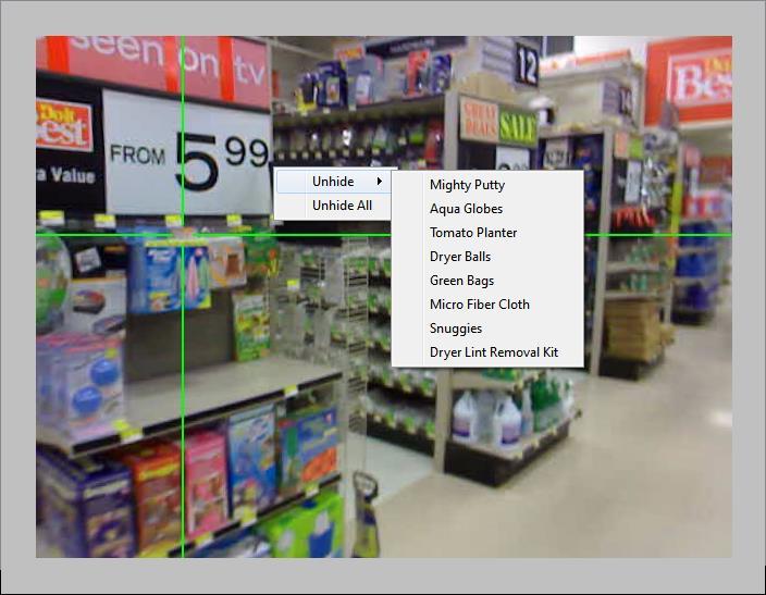
113 113

114 16.5 Sharing MAOIs, with multiple Segments or events The most efficient way to share a video and MAOIs with multiple data Segments or events is to first make the video file an Environment Video, and create the MAOI set on the Environment Video. It is possible to share an Environment Video, including MAOIS, with multiple Segments. Follow instructions in section 16.3 to make an Environment Video with MAOIs. If the beginning and end of the video file corresponds to the beginning and end of data Segments, select Configure Video Data from the context menu at a Segment node or whatever level above the segment node includes all events that will share the video and MAOIs. For example, to attach the video file with MAOIs to all files and all data Segments in the project, use the Participant File Node context menu. If Segments are divided into multiple events, each event will automatically use the appropriate section of the video and MAOI file. If the video beginning and end correspond to the beginning and end of one or more events (rather than an entire segment), the event node must be used, and the following procedure will need to be repeated for each such event. In the example, below, the Participant Files node has been selected, and the video with moving AOIs will be applied to all segments in the project. A Configure Video Data dialog will appear. If the video file corresponds to the beginning and end of the entire data Segment, set the Sync with button to Segment. If at an event node (the video file corresponds to the beginning and end of the event) set the Sync with button to Event. 114

115 Set the Video File radio button to Use Environment Video and make sure the proper video file name is specified. Next to Scale Gaze Data to Video: the same file name and frame number label should appear as that shown as Current Background: when data scaling was specified for the environment video (see section 16.3). Click OK. A Moving Areas of Interest node should now appear under each applicable event node. Fixations can be analyzed with respect to the moving areas of interest, and dynamic gaze and fixation data can be superimposed on the video with moving areas of interest also shown. 115

116 16.6 Creating MAOIs for individual events Once configured video data is associated with an event (see section 16.1) moving AOIs can be created for that event. In this case the MAOIs can be created only at the event node level and will apply only to that event. If the project type is Mobile Eye (csv file), this is the only way to create moving areas of interest. Right click an event node, and select Configure Moving Areas of Interest. A Configure MAOIs tab will appear in the Display Area showing the first frame of the video file corresponding to the selected node. Follow instructions in section 16.4 to create an MAOI set. When done be sure to click the Save and Close button on the Configure MAOIs tab. A Moving Areas of Interest node will appear below the event node. Fixations can be analyzed with respect to the moving areas of interest, and dynamic gaze and fixation data can be superimposed on the video with moving areas of interest also shown. 116

117 16.7 Fixation Sequence Analysis with moving AOIs (MAOIs) Fixations can be related to moving areas of interest, with associated statistics, in just the same way as they are related to stationary areas. There are two options available when computing Fixations with Moving AOIs. The user can choose to compute Fixations with respect to the scene image frame, or/and with respect to the moving areas of interests; these two options are described in the following sections. Once computations are complete, the fixation node can be expanded to show the fixation sequence and related nodes. The Fixation Sequence and Dwell information and statistics produced are the same as that described for stationary areas of interest in Sections 11 and Applying Fixations with Respect to Scene Frame to MAOIs When moving areas of interest are available, fixations can be determined either with respect to these moving areas; or with respect to scene image coordinate frame, as with stationary areas. This section addresses finding Fixations with respect to the scene image frame. In the case of head mounted optics, this means fixations will be considered to be periods during which gaze was stable with respect to the head mounted scene camera image, even though areas of interest may move within this image. In the case of table mounted optics this means fixations will be considered periods during which gaze was stable with respect to the stationary scene display. Note that the position of fixations, will not depend on Area of Interest positions. However, the fixation sequence analysis will determine when these fixation positions fall within one of the moving Areas of Interest. If desired, fixations can be computed first just as described in section 10.4, followed by selecting Find Fixation Sequence (Moving AOIs) from an appropriate node. Alternately, just select Find Fixation Sequence (Moving AOIs). If Find Fixation Sequence (Moving AOIs) is selected, a Configure Fixation Sequence for Moving AOIs dialog will appear to ask which type of fixations should be computed. For fixations with respect to the scene image frame, the subject of this manual section, set the radio button to Fixations with respect to Head. 117

118 Although the label reads Fixation with Respect to Head, in the case of ET3Space (or ASL EyeHead Integration) data or data collected with table mounted optics, this really means fixations with respect to a stationary display surface. This type of fixation sequence analysis can be selected from an Event, Segment, Participant (individual data file), or Participant Files (multiple data files) level. In the example below, it is being selected at the Event level, and the results will apply only to that event. A Fixation Detection Criteria dialog will appear. The fixation algorithm and parameters have been discussed in detail in section 10. Use default parameters or modify parameters appropriately, using the Advanced Configuration button if necessary, as described in section 10. If not using ET3Space (.ehd ) data, be sure to read section , and properly set the visual angle scale factor. Click OK when done. 118

119 A Fixations node should appear under the Default Event node. If there are multiple Moving Areas of Interest nodes available, then a Select Moving Areas dialog will appear and allow you to select which MAOI node to use. Fixations will now be assigned to the areas-of-interest that they fell within. A fixation node will appear under the appropriate event node (or nodes), and two new nodes will appear under the Fixations node, Fixation Sequence and Dwell nodes. Note, if you edit the AOI data that was used to generate these fixation sequence and dwell, you will need to rerun this analysis for your changes to take affect (on the fixation sequence and dwell). The Fixation Sequence and Dwell nodes both have an arrow sign to their left as well. Clicking on this arrow sign reveals additional data information (AOI Summary, Transition Table, Conditional Probability, and Joint Probability) with respect to fixations and dwells. 119

120 For a detailed explanation of the statistics reported see the explanation for stationary Areas of Interest in sections 11 and 12. Be aware, however, that since, in this case, areas of interest are moving with respect to fixation positions, it is possible for a given fixation to be within an area for only part of its duration Calculating Fixations with Respect to MAOIs When moving areas of interest are available it is also possible to define fixations as periods during which gaze remains stable with respect to one of the moving areas. If, for example, ocular smooth pursuit keeps gaze in a stable position on a moving target (and assuming the moving target is bounded by a moving AOI), that will be regarded as a fixation. In this case, note that fixations can only be defined when gaze is within a moving AOI. This type of fixation set appears as a node under a Moving Areas of Interest node. Caution: if computing fixations in this way it is important that moving area of interest precisely follow the image target, both in terms of position, and apparent size. Remember that the program will look for periods of gaze stability with respect to the moving AOI boundaries, not the actual target image. Gaze position is treated as a horizontal and vertical position relative to the MAOI bounding box. For example, gaze at any particular sample, may be 1/3 (0.33) the distance from the left edge of the bounding box to the right edge, and half (0.5) the distance from the top edge to the bottom edge. To compute these Fixations with respect to the moving areas, right-click on a Moving Areas of Interest node and select Find Fixation Sequence, or any node above that and choose Find Fixation Sequence (Moving AOIs). In the later case, the Configure Fixation Sequence for Moving AOIs dialog will appear, and the radio button should be set to Fixations with respect to AOIs. 120

121 The Fixation Criteria Detection will appear once again, allowing the user to set their desired parameters for defining fixations (see section 10). Two new nodes, labeled Fixation Sequence and Dwell, will appear under the Moving Areas of Interest node. Note that there is no Fixation node, since this type of fixation is only defined by association with a Moving Area of Interest. Expanding the Fixation Sequence and Dwell nodes will reveal additional data information (AOI Summary, Transition Table, Conditional Probability, and Joint Probability) with respect to fixations and dwells. The Fixation Sequence and Dwell information and statistics produced are the same as that described for stationary areas of interest in Sections 11 and 12. For periods during which gaze is not within any defined MAOI, fixations are computed with respect to the scene image frame (as discussed in the previous section), and fixation positions are reported with respect to the eye tracker coordinates. Fixations within MAOIs, on the other hand, have positions that are reported as a fraction of the horizontal distance from the left to right edge of the MAOI bounding box, and a fraction of the vertical distance from top to the bottom of the bounding box Playing the scene video with superimposed Gaze Trail and other information A scene video associated with an event can be viewed with a dynamic gaze trail and/or head map display from any event node. Fixations can be dynamically displayed on the video from fixation nodes; and areas of interest, along with a time line display showing the areas visited, can be displayed with the video from fixation sequence nodes. From an event node, right click to see the context menu and select Play Video with Gaze. If a video file has not already been associated with this event, a Configure Video Data Window will appear. 121

122 The video tab will open in the Display Area. The Configure Display pull down menu provides check boxes to enable Draw Options and Plot Options dialogs, and to enable a pupil diameter plot with moving time bar below the main display. The moving time bar (red line that moves from left to right) indicates the current position on the pupil diameter chart. If enabled, the Draw Options tab allows selection of the information to show over background image. Check Gaze Trial, Heat Maps, or both. A dialog window for adjusting the length and color of the gaze trail can be brought up by clicking the Gaze Trail Configuation button, and a dialog for heat map properties can be brought up by clicking the Heat Map Configuration button. The Plot Options tab, if enabled, allows adjustments to the pupil diameter display. The Viewer window includes the usual controls for play, pause, single step forward or back, advance to specified frame, and playback speed. A slide bar can be dragged to advance or back up through the video. There is also a pull down menu at the lower left of the main display with selections to record the video display as an avi file, or capture the current frame as bit map image. A full screen button at the lower right will toggle to a full screen display that omits the tree diagram, or back to the standard display. To see the same display with MAOIs also superimposed, select View Moving AOIs with Gaze Data from a Moving Areas of Interest node. 122

123 Select Play Video with Statistics from a Fixation Sequence node to also see MAOIs, and fixation trails. In this case and a AOI time plot showing when the various moving areas were visited by the subject. Using the Configure Display pull down menu, AOI Dwell Plots can be selected in place of Pupil Diameter. In this case the plot below the background image displays a time line plot showing when the various moving areas were visited by the subject. display shows a horizontal bar for each AOI with the AOI color indicating periods during which gaze was in that AOI. A moving time bar (vertical red line that moves from left to right) shows current time position on the plot Swarm video with shared stimulus videos and MAOIs Swarm Video over Shared Video and Swarm Video over Moving AOIs are available selections under the Group menu. Swarm Video over Shared Video is applicable if the same stimulus video is associated with multiple segments or events (for example, when the same stimulus video is shown to multiple participants). More specifically, it is usually applicable if data was gathered with table mounted optics, or EHI, as multiple subjects watched the same video presentation on a display screen. Gaze points for multiple events (usually multiple participants) are shown as multiple dots, each a different color, moving about over the shared stimulus video. See section for detailed instructions. Swarm Video over Moving AOIs is usually applicable when data was gathered by a head mounted eye tracker using only a head mounted scene camera. Note that in this case the scene video is different for every subject (or every event). Objects in the environment move about on head mounted scene camera image as subject s move their heads. Even if all subjects moved about in the 123

124 same environment, they all move differently, and the scene video recorded from the head mounted camera will be different each time. Moving Areas of Interest must be defined separately for each event. In this case it is not possible to swarm data from multiple events over a video because there is not a common video. The system does however calculate where gaze is with respect to the bounding box of each moving AOI. For example at the given time from an event start, a particular visual object in the environment, say a soft drink bottle, might be at a completely different position in the subject 1 video and subject 2 video. In each case, however, the system will know exactly where gaze was with respect to edges of the moving AOI defining the soft drink bottle outline in each video. If we have a static image showing the soft drink bottle and make a static AOI to define its outline, we can show the position of both subject 1 gaze and subject 2 gaze with respect to the static AOI on this image. This can be done for multiple Areas of Interest. Detailed instructions are in section Swarm Video over Shared Video When Swarm Video over Shared Video is selected from the Group menu, a selection chart appears labeled Select events that share same video. The user can select the events by checking individual event boxes, or higher level boxes, in a tree diagram. Checking Segment node, checks all of the events under it. Checking the Participants node selects all events in the project, etc. There are also Select all and Unselect all buttons. The Advanced button brings up a dialog that allows selection of events based on various criteria. The events can be automatically selected based on the name of the node, the first XDAT value in the event, or the configured background associated with the event. So, for example, it is possible to select all events for which the initial XDAT value is 1, etc. Either check the box corresponding to each event 124

125 that will be included, or use the Advanced button to specify display shows point of gaze for each selected event as different colored dot which moves about over the stimulus video. When data from many events are combined, it looks like a swarm of bees flying over the background image, and can provide a visual illustration of whether all subjects followed a similar gaze pattern (dots stay tightly grouped) or a variety of different patterns (dots tend to spread out over display). The Swarm Video over Shared Video is very similar to Swarm Video over Background discussed in section 15.1, but displays the gaze data with respect to video scene images rather than static background images. The viewer controls are the same as those discussed in section Swarm Video over Moving AOIs It is assumed that, for each event to be combined in a swarm, the same set of visual objects were defined by an MAOI set, on the stimulus video, and that Fixation Sequence has been computed for all each of these events. Before selecting Swarm Video over Moving AOIs proceed as follows to create a static image and static AOIs containing the visual objects of interest. From the Main menu select Configure Background Images; then, from the Configure Backgrounds tab, select Background Create single background. Select a static image showing the visual objects of interest. Note that the Extract Background Image from Video button can be used to select a frame from one of the scene video for use as the static image. Follow instructions in section 7 to configure the image. From the Main menu select Configure Areas of Interest (moving in background). A tab labeled Configure MAOIs in static background will appear in the display area. Next to Background:, at the top of the display, select the background created as described in the previous paragraph. Next to AOI set::, at the top of the display, use the pull down menu to select the MAOI set used for one of the scene videos. An Areas of Interest: list will appear to right of the display listing all the AOI names used in the selected MAOI set. Draw an AOI around one of the visual objects in the background. Follow the instructions in section 8.1 to draw either a rectangular or polygon area. The only difference is that the AOI properties box does not allow typing an AOI name. Rather, it has a pull down menu next to Name: that contains the list of MAOI file areas. One of these must be selected. The AOI must be the same type (rectangle or polygon) as the area with corresponding name in the MAOI set. Repeat the procedure to draw all the applicable AOIs on the static background, and be sure to click Save and Close when finished. Now select Swarm Video over Moving AOIs from the Group menu. Use the selection chart to select the desired Fixation Sequence Nodes. As with other Group displays, the Advanced button brings up a dialog that allows selection of events based on various criteria. Click OK to close the selection chart. As with other swarm displays, the viewer will show the gaze point from each event as a different colored dot. The viewer controls and selections are also the same as for other swarm displays. The difference is that gaze points will only be shown when they were within one of the MAOIs. 125

126 17 SceneMap Features (Requires SM License) The SceneMap feature can be used to significantly speed up analysis in cases where head mounted eye tracker optics are used to record data with respect to a head mounted camera, in environments where a separate head tracking system is not available or not practical. The SceneMap function will work best in environments where objects are primarily static, and where there are always significant image features (lines and edges) in the scene camera field of view. In other words, subjects are being tracked in a defined space with minimal moving objects. If some scene image objects do move with respect to the environment, their motion can be manually compensated for as described in Section. In order to use SceneMap features, it will first be necessary to use the eye tracker scene camera to capture a video of the environment within which participants will move about. A SceneMap Template must be placed within this environment in order for the environment to be mapped with ETAnalysis. (The template is available as a pdf file, usually in C:\ Program Files (86)\ Argus\ETAnalysis\Docs, and can be printed on standard printer paper.) The environment video should capture all visual objects in the environment that will be areas of interest (AOIs) (e.g., a box on a shelf for which gaze time statistics are desired). The SceneMap template should be placed close to these visual objects of interest but not covering any of their corners or vertices. The environment video should capture multiple views of each visual object of interest, as well as the typical viewpoints of participants. For instance, if participants will be sitting down and looking up at AOIs, your environment video should contain these upward viewpoints of the visual objects. For additional tips on creating an Environment video, see the separate Environment Map Tips document, accessible via the ETAnalysis Help menu and usually located under C:\ Program Files (86)\ Argus\ETAnalysis\Docs. SceneMap allows definition a single set of AOIs for an entire project, and will automatically apply these AOIs to each participant, despite the AOIs moving differently within each participant video Map Environment Open an environment video by selecting the toolbar button or selecting Open Environment Video from the File menu. The name of your environment video will appear under Environments, as a node in the Project tree: 126

127 Begin processing the environment file by computing its corresponding map and camera motion. Right-click on the Environment node and select Compute Environment Map and Camera Motion : In order for ETAnalysis SM to localize all contrast points within the video and later define AOIs in a known coordinate system, it must use the template corners as reference points. Therefore, it 127

128 will be necessary to initialize the corners of the target template in the first video frame. If the template is not visible in the first frame of the environment video, choose a different frame on which to start mapping (if the template is visible later in the video) or recreate the environment video with the template in your environment. To choose an alternate start frame, use the controls within with the Select frame at which to start mapping section. Note, only frames after this start frame will be processed so the start frame should not be too close to the end of the video or you will not have sufficient data for further processing. Once at an appropriate start frame, click anywhere within the inner black rectangle of the template. A new dialog will appear showing the automatic detection of the SceneMap template as in the following image. If the red rectangle approximately corresponds to the black region of the template (as in the image shown above), click OK to continue. If the automatically detected rectangle does not properly correspond, click and drag the corners of the rectangle to correct it, then click OK to continue. The environment will now be mapped and no interaction is required until mapping is complete. An estimate of the time required to map the environment video will be presented. The program recognizes contrast points in your environment, which are indicated by green and yellow circles. The green circles represent well-tracked contrast points that have a high confidence associated with them, while yellow circles indicate points that are in the process of being tracked and contain more uncertainty. 128

129 In the upper right corner of the video, ETAnalysis SM gives a confidence level of its scene recognition. The highest confidence is Best, followed by Good, then OK and finally Losing. If not enough contrast points are available, the system will show a Lost condition. Some Lost condition is acceptable, but high quantities of lost conditions are an indication of an unacceptable environment map. The environment mapping will run through the selected video two times. The Estimated Time Left includes both runs. This time can vary from environment to environment and is not just a function of the number of frames in the video; videos that contain long regions of Lost frames will process much more slowly than videos for which tracking is more successful. The mapping progress (fraction of frames processed each run) can be found under the video. Once mapping is complete, an Information pop-up will appear informing you of the overall confidence level of the mapping process. Usually anything above 75% is considered to be a good environment map, although it is difficult to generalize. 129

130 Upon completion of computing the environment map and camera motion, two new nodes, called Camera Motion and Environment Map, will appear in the project tree representing these data sets Define Areas of Interest Once a completed environment map has been saved, areas of interest (AOIs) can be defined within the environment. These will be the areas defining visual objects in the scene that will be the subject of gaze data analysis. The remainder of this section will focus on the process and tools needed to define these AOIs. To begin, right click the node labeled Camera Motion, and choose the "Define SceneMap Areas of Interest" option or click the corresponding button with the environment or camera node selected in the tree. OR The "Defining AOIs" tab will open in the Display Area. 130

131 This tab provides multiple tools that allow navigation through the video; the title of the tab Defining AOIs for EndCap_env_00000 (AVI) specifies the video within which AOIs are being defined. Below is a brief description of each button and its effect on navigating through the video. You may also use the scroll bar to navigate through the video. Play/Pause buttons Step Back/Step Forward buttons Steps backwards/forward with each click by the number of frames shown in the text box between these two buttons. Back to First Frame button Returns video to first frame upon clicking. Go to Selected Frame button navigates to the frame entered in the corresponding text section. Total number of frames shown after this, followed by time at each frame / total time of video. To create an AOI, begin by using the navigation tools described above to search through the environment video for a point in the video where the first AOI is fully visible. Once the object to be 131

132 defined is visible, make sure it is completely visible (shown completely within the video window). It is best not to start defining an AOI on the first video frame because this frame is the first frame processed and therefore its camera information may not be as accurate as later frames. When the AOI to be defined is fully visible, click the Add SceneMap AOI button located to the right of the video at the top of the Areas of Interest tab. The following window should appear. The above window shows the selected frame on the left and a second frame, some number of frames forward in the video, on the right. In order to define your AOI, it must be present in both images. Furthermore, in order for ETAnalysis SM to properly recognize an AOI, both Camera Status and Distance Status must show OK. If the images selected are within the frame and the Distance Status shows Too Close, then the images selected are too similar. This will not produce accurate results. Adjust the image viewed using the sliders below the frame images until an OK status is achieved. NOTE: If LOST shows up in as Camera Status, ETAnalysis SM was not able to properly map that specific angle. If there are excessive LOST status frames, re-creation of your environment video may be needed. Click OK when satisfied that both images clearly show the AOI to be defined. In the example shown, this will be the Micro Fiber Cloth. Next, the Area of Interest Selection window will appear. 132

133 The first image will populate in the upper middle frame. Clicking on the AOI s boundary, e.g. corners/perimeter, will teach ETAnalysis SM where the AOI is within the environment. In the example shown, we have a rectangular object, but ETAnalysis SM can define AOIs that have three or more vertices. Just be sure that they are entered in the same order in both frames around the AOI boundary. Each point will be given a sequence number and an outline of the area will be shown. Notice, in the following screen shot, that to the left and right of the top image, a zoomed in view of the images will appear. These views can help the user to properly recognize the points to be selected. To begin, select the upper left corner of the object (in the example, the Micro Fiber Cloth box). Then, continue on by selecting the upper right corner, lower right corner, and lastly the lower left corner. Once the points have been selected on the first image, click Go To Next Image. Repeat the process in the same order to select the corresponding points in the second image. A red line will indicate where the current point should be selected depending on the selection made in the first image. Right clicking on the image and selecting Delete Last Point can remove the last point drawn. 133

134 After all points have been selected, click Obtain More Frames. ETAnalsysi SM will now search through your environment video and select all frames for which the AOI is fully visible. Based on the points selected, ETAnalysis SM will predict where these points are in the subsequent frames. These points will show up in the populated frames list as small, numbered red crosshairs. 134

135 If all the red crosshair indicators for the current image seem to be correct, click Accept All Predicted Points. If one or two points need adjusting, change just those points by clicking Accept Current Predicted Point on the points that are accurate, and clicking the corrected vertex location on the frame where the predicted point is off. For instance, if the third point of a four vertex rectangle is off, select Accept Predicted Point for points one and two, click within the video frame on the lower right corner (which is the correct location for our current AOI) for point three, and then click Accept Current Predicted Point for point four. Then click on Next image to begin identifying the next frame. If you want to skip a specific image click Skip Image, and if you misclick a specific vertex click Clear Current Region to start over or Delete Last Point to re-do the last selected point. NOTE: All these options stated above are also available by right clicking your mouse within the active video frame. Once satisfied with AOI definitions, click Finish Now (assuming the video is not yet at its end). ETAnalysis SM will automatically reassign points to the remainder of the frames. Upon completion, an AOI Properties window will open. 135

136 Use this window to uniquely name the AOI, and to select a color and border width. In the example shown below, the name has been changed to Micro Fiber Cloth. Click OK. The AOI will now be shown throughout the video. Once the first AOI is complete, continue this process until all AOIs have been created. Below the Add SceneMap AOI button is a section where a list of defined AOIs will appear with a colored box next to their name. The colored box represents the AOI color in the video. The AOI can still be edited by clicking on its name and clicking the Edit button. This will cause the AOI Properties window to appear once again. To save the AOIs, click the Save & Close button. The AOI set will automatically be saved and applied to the project under the Camera Motion node. The AOI can be exported, so that they can opened in another project at a later time, by clicking the Export button. The location and file name can be changed when exporting. 136

137 After creating an AOI set, the project tree will have a newly created node, under the Camera Motion node, called Areas of Interest (if necessary, expand the tree to see this node) Track Head Motion Once the Environment has been processed and Areas of Interest have been defined, use ETAnalysis SceneMap to track the Head Motion for each participant Event. Note: All MobileEye participant video files must be processed through EyeVision before they can be used in ETAnalysis SM. It is recommended to remove the point-of-gaze crosshair from the participant video output before using the files within SceneMap. To remove the crosshair in EyeVision, go into the Scene Settings dialog (accessed via the Settings button in the Scene section of the main gui) and choose None for Cursor Type. Please refer to the Mobile Eye Manual for proper participant data and video creation. Open the participant data file as described in Section 5. The participant s head motion must first be computed in order to compute AOI positions within the participant video. There is an option to either compute head motion for the entire data file, or to parse the data into events (as described in Section 6) and track the head motion for each event. It is recommended that if there are sections of the video that will not be analyzed (e.g., time spent between tasks or when participant is not within the environment area), that the video be parsed into events containing just the portions of the video to be analyzed. Mulitiple events can be queued up to run the SM head tracking function in Batch mode as described in Section Tracking head motion for a single event us described below. To begin computing the head motion for the given participant video, right-click the Default Event node and choose Track Head Motion. Alternatively, click on the corresponding shortcut button; however, note that using the button will automatically track your participant using the project s configuration defaults for SceneMap Participant Tracking. 137

138 OR If Track Head Motion is selected from the context menu, a Configure Participant Tracking dialog will appear. Set the radio buttons for the type of system and lens used to collect data. Check the Assign AOIs from checkbox and be sure the proper AOI set is selected 138

139 Click OK. The Tracking Participant tab will open. Click Go, to begin tracking the participant. All of the buttons and features on this tab are the same as those on the Mapping Environment tab, described in a previous section. If, at the beginning of the video, the participant is not yet within the mapped environment, the confidence level will start with LOST. When the participant enters the environment, ETAnalysis SM should begin to successfully map the participant. If the participant data contains large sections before and/or after the participant is within the environment, you may choose to parse your participant data. If this is the case, you can right-click the Segment node and choose parse event, then parse the event by time or via the participant video. The event video must run through twice to complete the process. Estimated time to complete the head tracking operation for the entire event is shown at lower right. Upon completion, there will be two new nodes under the Default Event node. The Head Motion node contains the participant s head position and orientation data, and the Areas of Interest node contains the data for AOI positions in the participant s video. If necessary, expand all nodes to view the additional nodes. 139

140 To watch the previously created environment AOIs automatically attach in the participant video, rightclick the Areas of Interest node and choose View Areas of Interest with Gaze Data Track Head Motion - Batch processing (Multiple Events) Since the head tracking operation requires 2 play throughs of the entire event video, it can take a significant amount of time. A batch feature is therefore provided, making it possible to queue up multiple events for processing without user supervision. The user specify a set of multiple events. These data sets are put on a queue and as one finishes tracking the next on the queue is selected and begins tracking. This allows the user to leave the computer unattended, or continue on a different task while ETAnalysis SM tracks multiple participants (and/or multiple events) without supervision. Once participant files have been added to the project tree, right-click the Environment Map node and choose Track Multiple Participants. The check-box tree Select Events For Tracking Motion will appear. If you select a single participant s node (node with name ending in (EYD) or (CSV) ), it will in turn select all event nodes corresponding to that participant. To select all events in the project, check the topmost node or choose Select All. Use the Advanced button to select events based on XDAT values, if applicable, or manually select each desired Event. 140

141 Upon clicking OK, tracking of the first event checked will begin. The Tracking Participant tab will open. 141

142 After Run 2 of this event, the head motion computation for the event is complete, and the next event will begin tracking automatically. Upon completion of all queued events, the Batch Track Motion window will appear. Notice the status of processed events is Complete and shows the percentage of frames for which head motion has been computed in each case. This Percent Confidence (which can always be viewed in the More Info tab when the Head Motion node is selected) does not necessarily need to be close to 100%, depending on the data. Head motion information is needed only for frames during which the participant is looking within an AOI. If Head Motion was not computed for some of these frames, the positions of AOIs in these frames will be estimated using motion data for surrounding frames. If these estimates are inaccurate the AOIs in these frames can be manually adjusted, as described in Section Manually Edit Areas of Interest Due to imperfections in tracking participant motion or movement of AOIs from their original positions in the environment, some AOIs may need to be manually manipulated in participant videos. Here we describe how to correct the positions of AOIs in these cases. Right-click an Areas of Interest node and choose Edit Areas of Interest. 142

143 A new tab will appear called Editing AOIs.. The window is similar to that for defining regions in an environment, but with a few additional options. All Environment AOIs will be loaded into the participant video: 143

144 Below the Add SceneMap AOI button (which is more relevant to the Environment file) is a new button labeled Edit SceneMap AOI Positions. Underneath these two buttons are a few more options: Draw a rectangular AOI to manually manipulate. Draw a polygonal AOI to manually manipulate. Compute AOI positions from participant head motion data for the current frame (to undo manual changes in a frame). Go to previous frame in which AOIs were manually moved or computed from head motion information (positions in intermediate frames are estimated from these anchor frames). Anchor all AOIs in the current frame. Remove anchor from all AOIs in the current frame (calculate AOI positions from surrounding anchors). Useful for undoing a manual change. Go to next frame in which one or more AOIs are anchored. If any AOIs are selected (during manual editing) then it will go to the next anchor for a selected AOI. Save (backup) AOI data (AOI data will automatically be saved when tab is closed, this button is purely for backup purposes). Display help information regarding manually manipulating AOIs. Hover the mouse over a button at any time to view a brief description of the button. Click the Go to Next Anchor button to automatically jump to the first frame in which the participant was tracked. The display will show the environment AOIs at their positions in the participant video as computed from the head motion data. Since this is the first frame in which the participant location was found, the AOI positions will probably not be perfect, but will often snap into their proper positions if the video is advanced. On a frame for which head motion was not computed, AOIs are automatically available for manual manipulation. Each AOI will have a hatched pattern and white vertices, as shown in the example below. This display indicates that the AOIs can be manually manipulated because we do not have head motion information for this frame. To adjust an AOI, simple left-click and drag a vertex of the AOI as shown in the example, below, for for the Dryer Balls AOI. View the name of an AOI at any time by hovering the mouse within the AOI. When an AOI is adjusted, its fill color will turn from grey to the region color to indicate that the AOI is now anchored. All vertices of an AOI can be manipulated at the same time by CTRL+left-clicking the AOI: 144

145 In the example above the an AOI has been selected in this way. A blue rectangle appears around the AOI. Adjust all AOI vertices at once by adjusting this blue rectangle. For example, hover over the center right handle (circled above) and drag it to the right. Repeat for the left side of the AOI and adjust the top right vertex. Multiple AOIs may be adjusted as a group using a similar technique. Either CTRL+left-click each AOI you wish to adjust or CTRL+left-click and drag the mouse to create a rectangular over the AOIs you wish to select. In this case, all intersected AOIs, shown within a blue bounding box, will be selected, and can be adjusted in a group by manipulating the blue box. Sometimes it is necessary to manipulate an AOI even on frames for which head position information has been computed. In the following example a participant removes an object from the shelf. AOIs do not properly follow moving objects, and the AOI for this object remains at the position where the AOI would be located had the participant not moved it. It will need to be manually adjusted across several frames. Advance to the first frame for which the AOI position needs to be adjusted. Click the Edit SceneMap AOI Positions button. The Start Manual Mode window will appear with all AOIs checked. Hit the Uncheck All button and then check just the AOI (or AOIs) that needs to be adjusted. This will tell ETAnalysis SM which AOIs are to be manually manipulated. All the 145

146 remaining AOIs will continue to be computed automatically using the participant head motion computation. Click Continue to Select End Frame. The video slider will adjust to start at the current frame. Use the slider to advance to the last requiring manual adjustments and click the Mark End Frame button (where the Edit SceneMap AOI Positions button was located). The selected AOI will now appear hatched in the frames selected and can be manually adjusted. 146

147 Use the slider or the Step button to advance the video in appropriate increments and adjust the AOI as needed at each increment. Use of the gray area outside the image boundary to help with adjustments Analyze Results See Section 16.7 for description of computing fixations, fixation sequences and dwells along with their corresponding statistics (e.g., AOI Summary Table). The only difference is that fixation sequence and dwell nodes will be created under Head Motion Area of Interest nodes. Play back of video with gaze data is available from Event node context menus as Play Video with Gaze, from Head Motion nodes as Play Video, from Areas of Interest nodes as View Areas of Interest with 147

148 Gaze Data, and from Fixation Sequence nodes as Play Vdieo with Statistics. The video player and display options at the various levels are the same as those described in Section

149 18 Stimulus Tracking Feature (Requires ST License) If gaze data is collected from participants as they view a single display monitor, and if data is collected using a head mounted eye tracker with only a head mounted scene camera (no separate head tracker, and therefore, no ET3Space or EyeHead Integration function), then Stimulus Tracking can significantly improve the efficiency and ease of data analysis. It can make analysis of this type of data almost as convenient and efficient as if the data had been gathered from an eye tracker with desktop mounted optics. This advanced option requires an additional license. To benefit from the Stimulus Tracking tools in ETAnalysis ST, four stickers must be placed on the corners of the participant display monitor (or similar rectangular display region). These stickers are provided by ASL, with the Stimulus Tracking package, and are shown in the following image. Proper placement of these stickers is shown in the following image. They should not obstruct the view of any stimulus being presented to participants. 149

150 If using Paradigm to present stimuli to participants, please see the ETMobile ST Paradigm Configuration.pdf help document. To record the monitor display as the participant is tracked, please see the ScreenRecorder Configuration.pdf document. Note that the screen recorder is only required and should only be used if participants are interacting with the computer such that the display on the monitor is indeterminate (e.g., contains scrolling or video game responses which may be different for participant). If participants are watching pre-generated videos or looking at static images, Paradigm or a similar presentation tool should be used and individual stimulus files should be configured in ETAnalysis once per project as opposed to configuring an individual screen capture videos for each participant. In order to analyze gaze with respect to stimuli presented on a computer monitor, ETAnalysis must track the position of the computer monitor through each frame of the participant s scene video Track Monitor There are two options when tracking the computer monitor through a participant s scene video: 1. Parse file (typically by video or XDAT) into one event per stimulus and track the monitor in each event. 2. Track the monitor in the default event (entire segment), then parse to divide the segment into appropriate events. In the first case, it will be necessary to initialize the monitor corners (Section ) for each event. Option 1 may be the preferable option if participants move or turn away from the monitor between events, or if, for any other reason, there are long periods irrelevant data (that do not need to be processed) between events. This option will also be preferable if only one stimulus is presented in the participant file, so that there is only one event per file. 150

151 In the second case (option 2), the monitor corners need be initialized only once to allow tracking through the entire file. Although the monitor corners can typically be initialized with just a single button click (to approve automatically detected positions), this second option will probably be the most efficient for most scenarios. After tracking through the entire file and then parsing into events, the monitor positions will be automatically assigned for each parsed event Initialize Stimulus Tracking in an event To start the Stimulus Tracking process select Track Computer Monitor (A), or click the Monitor Tacking shortcut Icon (B) from either a Default Event node (option 2), or a parsed Event node (Option 1). A Tracking Monitor tab will open in the display window, and will first be used to approve or correct the initial estimation of the circle center positions at each corner of the monitor bezel. The initial estimation of the monitor area-of-interest (AOI) will be drawn on the video frame as shown in the example below (A). A B C 151

152 One or more corners of the monitor may be inaccurate due to other features in the video looking similar to the monitor targets (B). If any monitor vertex appears to be wrong, simply click and drag it to the correct center of the circular target. When all four points appear to be in the correct positions, hit the Play button to start tracking (C). Watch as the monitor is tracked through the video (or step away if it is a long video, and return when the play through is compete). If at any point a corner of the monitor AOI veers off its proper target, pause the video, adjust that corner (by manually grabbing and moving it) and hit play to restart tracking. These manual edits may also be done at any time after tracking has completed. In most cases, manual adjustments will not be necessary. When the process is complete a Monitor node will appear under each processed event on the project tree diagram Parse file into one event per stimulus For efficient analysis, it will be important to parse data into events such that each event represents a different stimulus presented to your participant. In the case of screen capture videos, it will usually be most efficient not to parse data and to leave the segment as a single Default Event. Parsing is described in more detail in Section View or Edit Monitor in Scene Video Right-click a Monitor node, and choose View Monitor in Scene Video (A) to view the monitor video. If the monitor track is incorrect for some frames and needs to be manually edited, instead of selecting View Monitor in Scene Video, select Edit/Track Monitor in Scene Video (B). Proceed to a video frame in which Monitor track becomes incorrect, as shown in the example below (C), and select Edit Monitor Position (D). Advance the video to next frame where monitor recognition is again correct, and choose Mark End Frame (E). The Monitor recognition outline will now be adjustable in intermediate frames. Most likely, depending on movement of monitor and length of frames that need to be adjusted, it will be necessary to adjust monitor recognition in only a small number of frames. The position of the monitor will be automatically estimated in frames between manual adjustments. Play the video to see the estimated positions in the intermediate frames. See ETAnalysis SM for Mobile Eye Tutorial or Configure Moving AOIs Tips documents for more details on manual adjustment of AOIs. In most cases the monitor positions should be accurate in all frames and will not require any manual adjustment. D B A C 152

153 E 18.2 Import and Configure Stimulus Each image and/or video presented to participants (or screen capture videos, when applicable) must be imported to the ETAnalysis ST project and then configured. Backgrounds and videos can be imported globally such that they are available to the entire project, as described in the next section (section ). Alternately the backgrounds and/or videos can be imported separately from the Configure Stimulus dialog available at each event. In either case, the Configure Stimulus dialog must then be used to map the background or video to the monitor outline determined for each event as described in the previous section. In other words the program must determine how the background or stimulus video background corresponds to the monitor boundary outline. This is described in section Add Stimulus Files to project To add static backgrounds to the project, go to the Configure menu and choose Background Image(s) or click the toolbar button. Once in the background configuration tab, select the Create New Background button (C) and then the Browse button (D) to select the first image file. C D 153

154 Then choose Create multiple backgrounds (E) and add remaining images (F). Hold down the control key to select multiple images in the File Open dialog. Then Save and Close (G) the Configure Backgrounds tab. E F To add canned videos to the project, open each presented video by selecting Open Environment Video from the File menu or clicking the toolbar button. Multiple files can be selected by holding down the control or shift key or clicking and dragging across desired files. If using screen capture videos, each participant will be configured to a separate video and these can just be selected in the Configure Monitor Stimulus dialog discussed in the next section Configure Stimulus for each Event In order to analyze gaze data with respect to stimuli, ETAnalysis ST needs to know which stimulus was presented during each event and where the stimulus was located with respect to the tracked corners of the monitor. For each event, right-click its Monitor node and choose Configure Monitor Stimulus. Note, when the event is selected, you can select the More Info tab to view a preview of the first frame of the event; this may be helpful when determining which stimulus corresponds to which event. This step does need to be performed for each event because the corners of the stimulus must be accurately defined once per event. If the stimulus is a video that began and ended at the beginning and end of a segment (usually the case if using a screen capture video), and if the data segment will be parsed into multiple events, do the Configure Stimulus procedure at the Default Event node before parsing into multiple events. The procedure will then need to be done only once for the segment, and the video will automatically be divided properly when the segment is parsed into multiple events. 154

155 In the Configure Stimulus dialog, choose the background or video file. If these files have already been added to the project (as described in the previous Section), choose the stimulus file from the corresponding pull down menu (A). Otherwise, choose the Load background image (B) or Video File Browse button (C, see Note) to select the file from your computer. For video stimuli, choose whether the video should be synchronized to the event or segment (D) (i.e., does the video start and stop with the entire file segment or with the parsed event); often, if it s a canned video it will be synchronized with the event beginning and end, and if it s a screen-capture video it will be synchronized with the segment. Note, if using canned videos, as opposed to screen capture videos, it is most efficient to add these to the project before this step (see previous section) and NOT to add them via the Video File Browse button on the Configure Stimulus dialog. Adding such videos globally, as described in the previous section, greatly simplifies configuring moving AOIs in the stimulus video and analyzing these moving AOIs in each event. The Use as project defaults checkbox (E) pertains just to this file information and, when checked, will set the default for the next configuration to the same filename and sync options (in the case of a video). After configuring your stimulus, a preview of the stimulus will appear in the More Info tab when the Monitor node is selected. B A C D E Left click the four corners of the stimulus in a frame of the participant s scene video, as shown by (A) on the screen shot below. The display will show a zoomed-in view of the area around the current mouse position to aid in the selection (B). The size of the dialog can be expanded (if there is room on 155

156 the screen), or scroll to view entire frame. If any of the four corners of the monitor or the stimulus is not visible in the currently displayed frame (by default the first frame of the event is displayed), then choose another frame via the Choose frame button (C). Make sure all four corners of the monitor are visible in the selected frame because the monitor position must be accurate in this frame; however, you are selecting the corners of the stimulus not the corners of the monitor. The corner currently being selected should be checked to the right of frame (D). Once selected, a red crosshair (E) will appear with initials corresponding to that corner (e.g., TR for Top Right ). To reselect a corner, select its radio button (D), to make sure that corner is active, and use the mouse to reselect the corner. C D A E B To expedite selection of stimulus file for each event in the project, it may be most convenient to configure events in order of the stimulus presented. In other words, configure all events where the Koala image is presented, with the Use as project default box checked, then configure all events where the Hidden Man video is presented, etc. This it will be necessary to select the corners of the stimulus for each event and update the stimulus file information only once for each stimulus. When configuring screen capture videos, make sure to select the corners of the displayed screen image in the scene video image (A). These corners may or may not line up with the inside edge of the 156

157 monitor bevel (B), the best way to determine where these corners fall is to browse to a video frame where the edges of the screen image are most visible (via button C). If some of the corners are underneath the monitor edge (i.e., cropped out of view by your monitor), then the calculated gaze in stimulus may be less accurate. It is best to make sure that you can see all corners of the presented screen image when using the screen-capture method for your stimulus video. A C B 18.3 Configure Areas of Interest in stimulus files There are three possible scenarios for configuring Areas of Interest for Stimulus Tracking projects: 1) static AOIs in background images, 2) moving AOIs (MAOIs) in canned videos, 3) moving AOIs in screen capture videos. For the first two options, see Sections 8 and 16.4, respectively. To configure moving AOIs in screen capture videos, first make sure the event has been configured to the screen capture video (previous Section). Then, right-click the Monitor node and choose 157

158 Configure Moving AOIs in Stimulus Video. Note that this option will only appear after the stimulus has been configured to a video file. If Moving AOIs have already been configured in the stimulus, the option will read Edit Moving AOIs in Stimulus Video. Proceed as in Section When using screen capture video, Moving AOIs will usually need to be configured for each event (assuming each event uses a different video). If all participants viewed the same video or image files, moving AOIs should need to be configured once per stimulus file and will automatically be applied to each Monitor node that was configured to that stimulus. It may sometimes be the case that each participant viewed the same set of objects, although they moved about differently on each scene video. Although MAOIs must be created separately for each, it may be important that each MAOI set have the same number of AOIs, with exactly the same names, so that Group analysis functions can be used. A feature is provided to make this task easier. After the first MAOI set is crated, when creating the subsequent MAOI sets, AOI names can imported from the first set to insure that exactly the same names are used. On the Configuring MAOIs.. tab, choose Import Names. Imported AOI names will appeared grayed-out in the AOI list until they are created. After drawing a rectangular or polygonal AOI, a dialog box will appear presenting each AOI name of the same type (rectangle or polygon) that has not yet been selected. Chose the appropriate name for the AOI being created Analyze Results Compute Fixation, Fixation Sequence and Dwell statistics Gaze data used in Stimulus Tracking projects is always data that has been recorded with head mounted eye tracker optics. This original gaze data specifies gaze with respect to the head, and fixations computed using this data consider fixations to be periods during which the eye is relatively stable with respect to the head (see discussion in section 10). This is the only kind of fixation that is computed in Stimulus Tracking projects. To compute fixation, right-click an Event node (or higher to compute for multiple sub-events at once) and choose Find Fixations. Follow the instructions in section 10. To compute Fixation Sequence and Dwell statistics select Find Fixation Sequence (Static AOIs) or Find Fixation Sequence (Moving AOIs) from a fixation node or higher, and follow the directions in section 11 and 12, or in section Note, however, that computation of fixations as periods of gaze stability with respect to MAOIs, is not available from Stimulus Tracking projects. As in all other project types, AOI Bar Plots can be viewed after fixation sequences have been computed (see Section 14.3), and data can be combined across events as described in Section View Gaze, Fixations, and Fixation Sequence Statistics, over Stimulus The participants gaze data, fixations, and fixation sequence statistics can be viewed either over the original head mounted scene camera video, or over the stimulus background or video file. 158

159 To view data over the original head mounted scene camera video, select Play Video with Gaze from an Event node, Play Video with Fixations from a Fixation node, or Play Video with Statistics from a Fixation Sequence node. Note that Play Video with Statistics will not show AOIs superimposed on the scene video, but in all other respects, these displays are the same as those described in section View the data overlaid on the stimulus file, to get a cleaner higher resolution view than from viewing gaze over the head mounted scene camera video. View data this way by selecting Play Gaze over Stimuls from an Event node, Play Fixations over Stimulus from a Fixation node, or Play Statistics over Stimulus from a Fixation Sequence node. In this case, Play Statistics over Stimulus does include the option to show Areas of Interest drawn on the background or video. See sections 14.4 and 16.8 for a description of the various display options and controls. In addition to the controls described in sections 14.4 and 16.8, a smoothing filter can be applied to the data when using Play Gaze over Stimulus, Play Fixations over Stimulus, or Play Statistics over Stimulus. To apply the smoothing filter, check the Smooth checkbox located on Draw Options tab. Three levels of smoothing are available, as determined by the low, medium, and high radio buttons. Smoothing will apply only to the display. It will not change the data table values or computed statistics. 159

160 19 Additional Features 19.1 Copy Project Settings from Another Project Some Project Settings may be relevant to multiple projects and therefore ETAnalysis includes a tool to copy these settings between projects. Settings that can be copied include: Event Parsing Criteria Fixation Calculation Parameters Pupil Analysis Settings Time Plot Settings Eye Tracker units to Degrees Visual Angle Background Images and Attachment Points Static AOI Sets and/or Moving AOIs in Static Backgrounds Background and/or AOI Correspondences Fixations in Moving AOIs Preferences (compute with respect to head or AOIs) Fixation 2D Plot Drawing Settings Heat Map Drawing Settings Gaze Trail Drawing Settings Fixations in Video Drawing Settings Advanced Batch Criteria SceneMap Environment Mapping Settings SceneMap Participant Tracking Settings Parallax Distances (Moving AOIs only) Stimulus Tracking Default Stimulus Settings To copy any or all of these settings from one project into another, choose Copy Settings from Another Project from the Configure menu. You will see the small dialog in the following image. 160

161 Choose the project file (with extension.aslrp) of the project that you wish to copy; this file will be located in the project folder with the same name. In most cases, you will probably want to just copy all settings. To copy all settings, choose Copy All Settings or OK, all settings will be copied and the dialog will close. To select a subset of all settings, choose Select Settings to Copy. You will see a checkbox for each Settings item relevant to your project type. Check the ones you d like to copy and hit OK Export data By using context menu Export selections, any numerical data can be exported to a text file or to an xml file that can be read by Microsoft Excel (version 2008 or higher). In most cases only data contained in the selected node are exported. For example, selecting Export from an event node will export only raw data for that event (not fixation data or fixation sequence statistics, etc., that may be in sub nodes). Both the contents of the Data window and More Info window are included. In the case of Excel, these are on separate sheets. The exceptions are file, fixation sequence, and dwell nodes. Exporting from a data file node exports all segments of raw data in the file. File information is included, but not the More Info pages from each segment. In the case of Excel, the file information is on one sheet, and each segment is on a separate sheet. Exporting from a fixation sequence node does include the statistics subnodes underneath it (each on a separate Excel sheet). Similarly, exporting from a Dwell node includes the subordinate statistics nodes. 161

162 It may sometimes be desirable to export data from multiple nodes to a single Excel spread sheet or text file list. This can be done from the File Export to Excel or File Export to Text File menu selections. Hovering the mouse over one of these selections shows a list of node types. Clicking on one of the node types brings up a tree diagram showing all the nodes of that type in the project. Each node of the tree is a check box. For example, clicking Fixations brings up a diagram like the one shown below. Checking a fixation node selects only that node. Checking a higher-level node selects all of the fixation nodes underneath it. The dialog also has a Select all button and an Unselect all button. When OK is clicked all selected fixation nodes will be exported to Excel, and in this case will all be listed on a single Excel sheet. Columns containing the file name, segment number, and event name are included so that the origin of the data in each row is specified. This works in a similar fashion for whichever type of node was selected. Contents of the More Info pages are not included. Only the data lists are exported. 162