Calculation of Unsteady Loudness in the Presence of Gaps Through Application of the Multiple Look Theory

Transcription

1 University of Windsor Scholarship at UWindsor Electronic Theses and Dissertations 2010 Calculation of Unsteady Loudness in the Presence of Gaps Through Application of the Multiple Look Theory Helen Ule University of Windsor Follow this and additional works at: Recommended Citation Ule, Helen, "Calculation of Unsteady Loudness in the Presence of Gaps Through Application of the Multiple Look Theory" (2010). Electronic Theses and Dissertations This online database contains the full-text of PhD dissertations and Masters theses of University of Windsor students from 1954 forward. These documents are made available for personal study and research purposes only, in accordance with the Canadian Copyright Act and the Creative Commons license CC BY-NC-ND (Attribution, Non-Commercial, No Derivative Works). Under this license, works must always be attributed to the copyright holder (original author), cannot be used for any commercial purposes, and may not be altered. Any other use would require the permission of the copyright holder. Students may inquire about withdrawing their dissertation and/or thesis from this database. For additional inquiries, please contact the repository administrator via or by telephone at ext

2 Calculation of Unsteady Loudness in the Presence of Gaps Through Application of the Multiple Look Theory by Helen Ule A Dissertation Submitted to the Faculty of Graduate Studies through the Department of Mechanical, Automotive and Materials Engineering in Partial Fulfillment of the Requirements for the Degree of Doctor of Philosophy at the University of Windsor Windsor, Ontario, Canada Helen Ule

3 Calculation of Unsteady Loudness in the Presence of Gaps Through Application of the Multiple Look Theory by Helen Ule APPROVED BY: Dr. Laura Wilber, External Examiner Northwestern University Dr. Nihar Biswas Department of Civil and Environmental Engineering Dr. Peter Frise Department of Mechanical, Automotive and Materials Engineering Dr. Edwin Tam Department of Mechanical, Automotive and Materials Engineering Dr. Colin Novak, Co Advisor Department of Mechanical, Automotive and Materials Engineering Dr. Robert Gaspar, Co Advisor Department of Mechanical, Automotive and Materials Engineering Dr. Thecla Damianakis, Chair of Defense School of Social Work September 28, 2010

4 DECLARATION OF ORIGINALITY I hereby certify that I am the sole author of this dissertation and that no part of this dissertation has been published or submitted for publication. I certify that, to the best of my knowledge, my dissertation does not infringe upon anyone s copyright nor violate any proprietary rights and that any ideas, techniques, quotations, or any other material from the work of other people included in my dissertation, published or otherwise, are fully acknowledged in accordance with the standard referencing practices. Furthermore, to the extent that I have included copyrighted material that surpasses the bounds of fair dealing within the meaning of the Canada Copyright Act, I certify that I have obtained a written permission from the copyright owner(s) to include such material(s) in my dissertation and have included copies of such copyright clearances to my appendix. I declare that this is a true copy of my dissertation, including any final revisions, as approved by my thesis committee and the Graduate Studies office, and that this dissertation has not been submitted for a higher degree to any other University or Institution. iii

5 Abstract Experimental studies have shown that for short gaps between 2 to 5 ms, the perceived loudness is higher than for uninterrupted noise presented to the ear. Other studies have also shown that the present temporal integration models for the calculation of time varying loudness do not adequately account for short duration phenomena. It has been proposed that the multiple look approach is a more applicable method for describing these short term circumstances. This approach breaks a sound into small durations or looks having length of 1 ms which allows for the intelligent processing of the looks and decision making depending on the nature of the stimulus. However, present technologies (i.e. FFT) are not adequate to deal with short duration sounds across the entire frequency spectra. A compromised approach is taken here to account for perceived loudness levels for sounds in the presence of gaps while using an integration model. This approach is referred to as a multiple look gap adjustment model. A model and software code was developed to take a recorded sound presented to the ear and process it into individual looks which are then examined for the presence of gaps ranging in length between 1 to 10 ms. If gaps are found, an appropriate gap adjustment is applied to the sound. The modified stimulus is subsequently evaluated for loudness level using a model which relies on temporal integration. The multiple look model was tested using several sounds including mechanical and speech sounds and was found to perform as intended. While recommendations for improvement and further study are included, the application of the model has shown particular merit for perceptional analysis of sounds involving speech. iv

6 Dedication I would like to dedicate this Doctoral dissertation to my Mother, Ivi Ule, and in loving memory of my father, Janez Ule. Also included are the friends closest to my heart. Thank you for all of your love, support, and sacrifice throughout my life. v

7 Acknowledgments I would like to acknowledge the inspirational instruction, guidance and support of my co advisor Dr. Colin Novak for whom I could not have completed this effort without his assistance, tolerance, and enthusiasm. I would also like my co advisor Dr. Robert Gaspar who has always had time to listen to my thoughts, concerns and desires, no matter how elementary. My sincerest thanks are given to my other dissertation committee members, Dr. Peter Frise, Dr. Edwin Tam, Dr. Nihar Biswas and the external examiner, Dr. Laura Ann Wilber. Heartfelt gratitude is extended to all my friends for their support during this period of my life, especially my long time friend Paul Fedory for his guidance and expertise in computer programming languages. Acknowledgement is also given for the generous support and assistance to my academic pursuits by Bruel & Kjaer. vi

8 Table of Contents DECLARATION OF ORIGINALITY... III ABSTRACT... IV DEDICATION... V ACKNOWLEDGMENTS... VI LIST OF FIGURES... IX LIST OF TABLES... XI NOMENCLATURE... XII I INTRODUCTION... 1 II BACKGROUND ANATOMY OF THE HUMAN AUDITORY SYSTEM Outer Ear Middle Ear Inner Ear CHARACTERISTICS OF LOUDNESS MODELING LOUDNESS III LITERATURE SURVEY LOUDNESS MODELS Stationary Loudness Models Unsteady Loudness Models LOUDNESS USING TEMPORAL INTEGRATION RESEARCH SUPPORTING MULTIPLE LOOK APPROACH FOR LOUDNESS SUMMARY IV THEORY TEMPORAL INTEGRATION MULTIPLE LOOK UNSTEADY LOUDNESS MODEL V APPROACH PROPOSED MODEL TEST PROCEDURE VI DISCUSSION OF RESULTS STATIONARY PURE TONE SOUNDS STATIONARY MECHANICAL SOUNDS TIME VARYING (UNSTEADY) SOUNDS VII CONCLUSIONS AND RECOMMENDATIONS CONCLUSIONS CONTRIBUTIONS vii

9 7.3 RECOMMENDATIONS BIBLIOGRAPHY REFERENCE A REFERENCE B REFERENCE C VITA AUCTORIS viii

10 List of Figures Figure 1: (a) Schematic Illustration Demonstrating the Concept of Frequency Masking where One Sound Component is Masked by a Lower Amplitude Sound and (b) Schematic Illustration Temporal Masking where a Brief Sound Followed by a gap and then a Second Sound is Masked (Defoe, 2007) Figure 2: ISO 226:2003 Equal Loudness Contours which illustrate the extreme frequency dependence on perceived loudness (International Organization for Standardization, 2003) Figure 3: Schematic of the ear showing the main anatomical components of the outer, middle and inner ear (Science Kids) Figure 4: The transfer function, or frequency response, of the outer ear, including the resonance effects of the auditory canal at approximately 4 khz (Everest & Pohlmann, Master Handbook of Acoustics, 2009) Figure 5: Schematic of the cochlea stretched out showing the path of excitation through the cochlear fluid and along the basilar membrane (Hearing Aids Central.com) Figure 6: Relative position of excitation along the basilar membrane with respect to frequency. Low frequency excitation is located at the base of the membrane while high frequency excitation is found at the apex near the round window (Howard & Angus, Acoustics and Psychoacoustics, 2006) Figure 7: a) Idealized critical band filter envelope of excitation along the basilar membrane showing an assumed frequency bandwidth shape, b) idealized bank of several critical filter envelopes (Howard & Angus, Acoustics and Psychoacoustics, 2006) Figure 8: a) Three sounds having the same sound pressure level but varying bandwidths centred about 1 khz, b) Subjective loudness for equal sound pressure levels showing an increase in loudness for bandwidths greater than 160 Hz (Everest & Pohlmann, Master Handbook of Acoustics, 2009) Figure 9: Effect of duration on the perceived loudness for a steady tone where the loudness of the tone linearly increases for durations up to 200 ms after which the loudness becomes steady (Howard & Angus, Acoustics and Psychoacoustics, 2006) Figure 10: Schematic of Specific Loudness Plot, or Loudness Value per Critical Bark Band measured in sone. Also Illustrated is the Area under the Specific Loudness Curve N which is Directly Proportional to the Total Perceived Loudness (Bruel & Kjaer) Figure 11: Masking patterns of narrow band noise centred at 1 khz with a bandwidth of 160 Hz at different levels LCB (Bruel & Kjaer) Figure 12: Comparison of Zwicker s Critical Bandwidths to Glasberg and Moore s Equivalent Rectangular Bandwidths which demonstrate the low frequency errors resulting from Zwicker s listening experiments (Seeber, 2008) Figure 13: Perceived difference in sound level in db of two pulses with varying separation times and a single pulse showing an increased detectability for shorter separation times in ms (Viemeister & Wakefield, 1991) ix

11 Figure 14: Schematic illustration of Viemeister s experiment where pip signals are presented individually and simultaneously within two 10 ms gaps in the presence of a varying masker noise signal (Viemeister & Wakefield, 1991) Figure 15: Graphical representation of the transfer function representing the effects of the outer and middle ear on the time waveform input. The result of this filter is a representation of the sound at the cochlea (Moore, Glasberg, & Baer, A Model for the Prediction of Thresholds, Loudness and Partial Loudness, 1997) Figure 16: Sinusoidal representation of a 1 ms WAV file comprised of 32 samples which are given by hexadecimal values. Defined are the amplitudes for the Peak and RMS pressures of the sound wave Figure 17: Flow chart illustrating the proposed model from input of WAV file, conversion to 1 ms looks and search and adjustment procedure for the presence of gaps. The adjusted file is subsequently reversed back to a WAV file format suitable for the calculation of loudness Figure 18: Photograph of the experimental set up in the Semi Anechoic room showing the Bruel & Kjaer acquisition system, amplifier loudspeaker and microphone. The test sounds are generated by the PULSE sound generator and played by the loudspeaker and subsequently recorded through the microphone. The acquisition system then prepares the WAV file for the multiple look gap correction and loudness programs Figure 19: Time domain plot for the 90 db sinusoidal test sound without the modifications of inserted gaps in the signal Figure 20: Time domain plot for the 90 db sinusoidal test sound with the addition of inserted gaps in the signal with position and gap durations as specified in Table Figure 21: Output of the multiple look program which shows the number of gaps found in the 90 db gapped input file and the corresponding durations. Also given is the calculated loudness level using the integrated Cambridge model Figure 22: Time domain plot for the white noise test signal without the modifications of inserted gaps in the signal used for the calculation of loudness level with and without the multiple look model Figure 23: Time domain plot for the white noise test signal with the addition of inserted gaps in the signal with position and gap durations as specified in Table 4 used for the calculation of loudness level with and without the multiple look model Figure 24: Time domain plot for the warble sound used for the calculation of loudness level with and without the multiple look model Figure 25: Time domain plot for the recorded diesel engine sound used for the calculation of loudness level with and without the multiple look model Figure 26: Time domain plot for the spoken sentence, Suzie sold seashells by the seashore, chosen for its smooth cadence and expected lack of gaps Figure 27: Time domain plot for the spoken sentence, Clickity clack, the train went down the track, chosen for its rougher cadence and expected gaps in the signal x

12 List of Tables Table 1: Zwicker's 24 critical bands having unit of Bark and the corresponding bandwidth and centre frequencies having units of Hz 27 Table 2: Evolution of the significant work leading to the development of both stationary and unsteady loudness models, including the significance of each milestone. 40 Table 3: Detection correction levels for applied for corresponding gap durations to the 1 ms looks 71 Table 4: Position in signal duration having inserted gap, the length of the gap and corresponding adjustment 82 Table 5: Loudness level for 1000 Hz sinusoidal signals without inserted gaps calculated using DIN 45631, Cambridge model and with multiple look gap correction model 83 Table 6: Loudness level for 1000 Hz sinusoidal signals with gaps inserted calculated using DIN 45631, Cambridge model and with multiple look gap correction model 83 Table 7: Loudness levels for steady mechanical sounds (white noise, warble and diesel) calculated using the Cambridge model and multiple look gap correction model. 88 Table 8: Loudness levels for time varying sinusoidal sweep and speech sounds calculated using the Cambridge model and multiple look gap correction model. 91 xi

13 Nomenclature AGC automatic gain control ANSI American National Standards Institute db decibel CPB constant percentage bandwidth DIN Deutsches Institut fur Normung DSP Digital Signal Processing ERB Equivalent Rectangular Bandwidths f T Frequency of test tone F represents the fraction of the difference between the summation of all the loudness within a given band and the maximum band loudness FFT Fast Fourier Transform h r height of water in container (from example in Chapter 4) h r0 initial height of water in the container (from example in Chapter 4) h r (t) response to a sound with duration t (from example in Chapter 4) HATS head and torso simulator Hz Hertz ISO International Standards Organization khz Kilohertz, 1000 Hertz l rate of water leaking out (from example in Chapter 4) l T level of test tone ms milliseconds, 1/10 second N loudness ns nanoseconds R rate of rain (from example in Chapter 4) RPM revolutions per minute S loudness Sm maximum loudness S t total loudness SPL sound pressure level STEP spectral temporal excitation patterns t duration (from example in Chapter 4) t I integration time constant (from example in Chapter 4) TVL time varying loudness WAV Windows Wave (audio format/file extension) τ leak rate (from example in Chapter 4) xii

14 I Introduction The ability to hear and discriminate sounds is a critical sensory mechanism in humans as it enables them to communicate and to react to auditory stimuli within their environment. Communication is necessary for the maintenance of social relationships and the ability to detect and analyze sounds within the environment. It is critical to an individual s ability to understand its surroundings and to its overall quality of life. The physical manifestation of sound is that of vibrations of air molecules propagating through a medium. The human auditory system has the complex task of transforming this sound into something meaningful. The auditory system is a complex one for which much is still not understood in regard to the extensive processing of the physical stimulus of sound into a psychoacoustic perception of the stimulus. From an engineering perspective, the goal is often to finding the source mechanisms of a sound in the hope of altering them to either attenuate the noise or improve its quality from a perceptional perspective. The latter is referred to as the science of psychoacoustics or sound quality. In order to perform this task adequately it is also important that engineers understand the mechanisms of the human auditory system that influence these perceptions; that is, the relationships between the sound characteristics entering the ear and the perceptional sensations which they produce. Unfortunately it is difficult to understand both what the auditory system does and how it works. This is because the perceptional components of hearing a sound cannot entirely be explained by a simple understanding of the anatomy of the auditory system. Much of what is known about the perception of sound has been surmised by scientists 1

15 and engineers through psychophysical experiments for which the results have been used to model the perception and discrimination of sound. It is from these observed results that engineers have developed the mathematical models to predict the sound quality attributes of sounds. That is, they attempt to predict the perceived sound quality of a sound in the hopes of either determining a best sound from an array of product samples or perhaps to modify the sound to improve its quality. The most fundamental of all of the psychoacoustic metrics is loudness, a model for which many other metrics rely on for the basis of their calculation algorithms. Loudness is said to be a metric which closely matches the perceived intensity of a sound, however, this should not be confused with the physical quantity of sound intensity. Loudness is a psychological quantity measured by a human listener. On physical grounds alone, one expects that loudness should be different from intensity because the ear does not transmit all frequencies equally, i.e. it does not have a flat frequency response. (Hartmann, 1998) This nonlinearity in frequency is due to the geometry of the outer ear, resonances within the human ear canal and bone conduction. This results in a transfer function having resonances in the 3 khz to 12 khz frequency range. In other words, the magnitude of the acoustic stimulus input to the nervous system does not depend on a physical quantity of intensity alone and is instead largely frequency dependant. It is this fact which has lead to the development of the equal loudness contours first plotted by Fletcher and Munson at the Bell Laboratories (Fletcher & Munson, 1933). Another characteristic of loudness which involves frequency is frequency masking. Here, a sound or a frequency component of a lower amplitude sound is covered by another sound, or component of a sound with a similar frequency makeup. If a sound is unsteady in nature, another type of masking which can occur is called temporal or time masking. This can occur 2

16 when one sound, or component of a single sound, follows very closely after another in time. Figures 1(a) and 1(b) are schematic illustrations of frequency and temporal masking respectively (Defoe, 2007). The concept of temporal masking will be shown to be a very important component of this dissertation as it is associated with the perception of loudness for unsteady sounds. Figure 1: (a) Schematic Illustration Demonstrating the Concept of Frequency Masking where One Sound Component is Masked by a Lower Amplitude Sound and (b) Schematic Illustration Temporal Masking where a Brief Sound Followed by a gap and then a Second Sound is Masked (Defoe, 2007). Examination of the standardized ISO 226:2003 equal loudness contours given in Figure 2 illustrates the frequency dependence on the perception of sound due to the nonlinearity of the human auditory system at the low and high frequency extremes. The initial equal loudness contours which were later standardized were developed using jury testing techniques. For this, pure tones sounds were played to jurors who were asked to rate the loudness of successive tones at varying sound pressure amplitudes and frequencies compared to a 1000 Hz reference tone. The unit given to loudness on the equal loudness plots is the phon (pronounced as fawn). The reference line for the equal loudness contour is defined as the 40 phon line. For this plot, a 1000 Hz tone will have both a loudness of 40 phons and a sound pressure level of 40 db. As the frequency is decreased it is observed that the equal loudness contour for the 40 db line begins 3

17 to slope upwards illustrating a decrease in ability of the human ear to perceive sounds at these lower frequencies. A similar trend is illustrated as the frequency increases above 1 khz. The exception to this is a dip or enhanced acuteness to sound within the frequency range of approximately 4000 Hz. This is due to resonances within the human ear canal which act as a quarter wave resonator. Examination of the 40 phon line at 100 Hz shows that the sound pressure level of a sound would need to be approximately 65 db to sound as equally loud as the 1000 Hz at 40 db. Figure 2: ISO 226:2003 Equal Loudness Contours which illustrate the extreme frequency dependence on perceived loudness (International Organization for Standardization, 2003). 4

18 Loudness in phons can also be expressed as loudness level with the unit of sones where the 40 phon line represents 1 sone. For an increase in loudness by 10 phons, a double in loudness level is realized. For example, 40 phons is 1 sone, 50 phons are 2 sones, 60 phons are 4 sones etc. It should be noted that the representation of loudness using the equal loudness contours is rather simplistic in that it is a representation of pure tones only and not of more realistic complex sounds found in real life experience. For the estimation of loudness for real sounds, complex loudness models are needed. These models are divided into two fundamental types, being loudness models for stationary or steady sounds which do not change with time and more complex non stationary models used for the calculation of loudness of unsteady sounds. Several calculation techniques for both types can be found in the literature and are discussed in greater detail in Chapter 3. It should be recognized that the mechanisms underlying the perception of loudness are not all fully understood and that these models are only best approximations and are still fought with uncertainties and assumptions. The focus of this dissertation is on the more complex determination of loudness for unsteady sounds. To date, the generally accepted approaches to the calculation of unsteady loudness use the method referred to as temporal or long term integration where the intensity of the unsteady signals are integrated over time. Psychoacoustic studies have found this method to be acceptable for sounds which do not change significantly over durations of approximately 100 ms or longer. However, it has been known for many years (Exner, 1876) that the absolute thresholds of sounds are strongly dependent upon duration as well as frequency. Experiments have shown that the perceived absolute thresholds are increased for sounds which are short in duration or in the presence of gaps. The use of temporal integration methods cannot account 5

19 for the short duration data, and therefore, cannot be considered to be good predictors of loudness for all signal types. An alternative theory which is thought by some to be a better representative auditory model of the human hearing system is called the multiple look approach. The premise of the multiple look theory is that the auditory system takes many samples or looks of a stimulus and stores them into memory for later processing. The specific processing performed is dependent on the makeup of the signal contained in the successive look. For the case where gap or burst of information is present, the short term looks are processed immediately as an auditory perception. If the signal is steadier in nature, the looks are instead stored for a longer period and then processed as an integrated signal over time, synonymous with the concept of a leaky integrator model. The caveat of the multiple look approach is that it cannot be adequately implemented using present day technology over the full auditory frequency range given the limitations of present day digital signal processing techniques. That is, the DSP cannot adequately sample short duration signals with a low enough frequency resolution to cover the full auditory range. The objective of this work is to develop an alternative model which will account for the hearing phenomena demonstrated by the experiments supporting the multiple look theory while at the same time be viable to implement in light of the present day limitations of signal processing capabilities. The proposed model is a hybrid multiple look approach which uses level correction factors in conjunction with temporal integration methods in order to adequately represent the perceived loudness levels in the presence of gaps in a stimulus signal. 6

20 In addition to the solution statement above, the scope leading to the objective is to ensure flexibility and wide use adaptability of the model. As will be detailed further in this report, it is intended that the multiple look model developed will be integrated into existing and future loudness models using integration theory. As such, the model developed here should be easy to integrate into any of these loudness models. While this work is focused on the hearing phenomenon of gap detection, the algorithm should be easily adaptable to other attributes such as burst detection. The code should be open and allow for modifications to its parameters and correction values in order to accommodate new empirical data in the future. Finally, the method developed model should be well suited to be used for other psychoacoustic metric such as speech intelligibility. The layout of this dissertation is as follows. Given the nature of the material presented in the literature review section, some background information is first provided in Chapter 2. The intent is to provide fundamental information in regard to how the auditory system functions as well as a more thorough description of the mechanisms related to the perception of loudness and how it is modeled. This information is necessary for the non audiologist in preparation for Chapter 3 which is a traditional presentation of the literature review which identifies the present state of art. Chapter 4 provides the background theory of the calculation processes which is necessary to bridge the gap between Chapter 2 and the methodology details given in Chapter 5. A detailed description of the multiple look gap correction model developed in the dissertation as well as the experimental setup is given in Chapter 5 followed by a presentation of the results in Chapter 6. Finally, a discussion of the conclusions and recommendations for future work will be provided in the final chapter. 7

21 II Background Acoustics is a well developed science of the study of sound from a physical perspective. It deals with the quantification of the physical parameters of sound power or sound pressure. Psychoacoustics is the study of how we perceive sounds. This includes the quantification of how good or how bad a noise source sounds is perceived to be by an individual listener. In order to study psychoacoustics, it is necessary to first understand the physiology and workings of the human ear. This chapter will describe the main anatomical structure of the human ear as well as how these mechanisms are related to how humans perceive sounds. Also described will be the psychoacoustic metric of loudness including the link between the functional components of the ear and this perceptional metric. The discussions on loudness will include models that are for both stationary sounds which do not change with time as well as unsteady sounds. It should be noted though that much of the present understanding of hearing perception is based on listening experiments where controlled sounds are introduced to listeners and their responses are correlated to the inputs. While the responses to these experiments cannot often be described by the physiology of the hearing system in term of physical means, they do provide a foundation to the understanding of hearing perception and psychoacoustics. 2.1 Anatomy of the Human Auditory System The anatomy of the human ear is divided into three fundamental sections as illustrated in Figure 3. These three sections are comprised of the outer ear which acts not only as a receptor devise but has other important functions including sound localization. The middle ear acts as a mechanical amplifier of the sound waves which reach the tympanic membrane, or eardrum. The inner ear performs many of the functions which dictate hearing perception. A more detailed description of each of these components which make up the ear is given below. 8

22 Figure 3: Schematic of the ear showing the main anatomical components of the outer, middle and inner ear (Science Kids) Outer Ear The outer ear consists of the pinna, concha and the auditory, or ear canal. The pinna is the external tissue which is comprised of grooves and depressions. The pinna acts as a noise collection devise which has a similar effect to holding your open hand around your ear to direct noise into the ear. The main depression or cavity before the auditory cannel is the concha. Together the pinna and concha aid in the effort of sound localization to determine the front to back and up and down positioning of a sound source. The auditory canal directs the sound to the tympanic membrane while at the same time offering some protection to the membrane. The approximately 25 mm long auditory canal, as well as the pinna and concha modify the frequency response of incoming sounds as shown in the transfer function in Figure 4. The auditory canal has 9

23 the most significant effect by amplifying sounds by several decibels in vicinity of the 4 khz frequency range. It does so by acting as a quarter wave resonator, very much like an organ tube. The sound waves strike and cause the tympanic membrane, a very thin elastic boundary separating the outer and middle ear, to vibrate. The displacement of the ear drum is 10 3 nm at threshold of hearing (about 3/100 diameters of the hydrogen atom) and 10 3 nm at the threshold of pain. Figure 4: The transfer function, or frequency response, of the outer ear, including the resonance effects of the auditory canal at approximately 4 khz (Everest & Pohlmann, Master Handbook of Acoustics, 2009) Middle Ear The middle ear is comprised of three tiny bones called the ossicles which is made up of the malleus, the incus and the stapes. Just as the malleus is fixed to the tympanic membrane, so is the stapes to the oval window at the boundary to the inner ear. The purpose of the middle ear is to transmit the excitation of the tympanic membrane to the relatively incompressible cochlear fluid inside known as perilymph without significant energy loss. Given that the energy transfer is from air to a liquid, a significant impedance change must be overcome. In this case, the impedance ratio is 10

24 approximately 4000:1. This is accomplished in two ways. The first is the mechanical advantage realized from the ossicles which act as three mechanical levers. The second is from the area difference between the tympanic membrane and the footplate of the stapes on the oval window. As a result, the pressure increase from the input to the malleus at the tympanic membrane to the output at the foot of the stapes into the oval window is approximately 33.8 times. A second function of the middle ear is to protect the auditory system from excessively loud sounds. This is accomplished by two muscles called the tensor tympani and the stapedius which contract and stiffen the ossicles system when exposed to sounds in excess of 75 db pressure level. This phenomenon is known as the acoustic reflex and provides approximately 12 to 14 db of attenuation for frequencies below 1000 Hz Inner Ear The inner ear is comprised of a snail shaped bone structure which is about the size of a pea called the cochlea. The function of the cochlea is to convert the mechanical vibrations induced into the cochlea by the stapes at the oval window into nerve impulses or firings to the brain to be processed into acoustic impressions. The fluid filled cochlea is approximately 25 mm long and coiled about 2.75 turns. It is divided along its length by two membranes called Reissener s membrane and the basilar membrane. Shown in Figure 5 is a schematic of the cochlea stretched out which shows the position of input vibration at the stapes into the cochlea. This energy then propagates along the length of the cochlea then down and back again to the round window causing an outward movement resulting in a pressure release. It is on the basilar membrane that standing waves are set up along its length and are positioned 11

25 depending on the frequency of the pressure excitation. As shown in Figure 6, low frequency excitations are located near the end of the basilar membrane while high frequency excitation has maximum amplitude at the apex near the oval window. Figure 5: Schematic of the cochlea stretched out showing the path of excitation through the cochlear fluid and along the basilar membrane (Hearing Aids Central.com). Figure 6: Relative position of excitation along the basilar membrane with respect to frequency. Low frequency excitation is located at the base of the membrane while high frequency excitation is found at the apex near the round window (Howard & Angus, Acoustics and Psychoacoustics, 2006). 12

26 Located along the basilar membrane are thousands of hair like structures containing tiny hair bundles called stereocillia. When waves are set up on the basilar membrane, the stereocilla are bent which in turn results in discharges of electrical signal which initiate neural discharges to the auditory nerve and then to the brain. The firing of a neural discharge will initiate the firing of an adjacent fibre. It is believed that the loudness of a sound is proportional to the number of nerve fibres excited and repetition rate of the firing. It should be noted that a thorough understanding of how the inner ear and brain works is not yet known (Everest & Pohlmann, Master Handbook of Acoustics, 2009). For a future understanding of loudness perception, it should be understood how the excitations along the basilar membrane relate to perceived frequency. The response is very much like a constant percentage band filter on an acoustic analyzer where the frequency response is divided into bands or envelopes with the width of each envelope increasing by the same percentage of the centre frequency of the band. For a one third octave analyzer, the width of each frequency band is a constant 23 percent of the band s centre frequency. The response along the basilar membrane acts in a very similar manner. Here, each band is often referred to as critical band (also referred to as Bark bands). Other theories exist which differ somewhat in the shape of the bandwidth windows. One such alternative is given by Glasberg and Moore who defined the bandwidths by Equivalent Rectangular Bandwidths (ERBs) (Glasberg & Moore, 1990). More detail to the different approaches is given in Chapter 3. Shown in Figure 7 is an idealized frequency response on the basilar membrane for a localized frequency excitation as well as a broadband excitation. The exact widths and locations of the 13

27 critical band centre frequencies is still unknown and gives rise to the different theories and approaches for the calculation of loudness. Figure 7: a) Idealized critical band filter envelope of excitation along the basilar membrane showing an assumed frequency bandwidth shape, b) idealized bank of several critical filter envelopes (Howard & Angus, Acoustics and Psychoacoustics, 2006). 2.2 Characteristics of Loudness As described in Chapter 1, the work done by Fletcher and Munson (Fletcher & Munson, 1933) on the equal loudness curves (Figure 2) provided the foundation for the later development of models for the calculation of loudness. The unit for loudness which corresponds to the subjective impression of the intensity of a sound is the sone. The sone is defined as a subjective unit because a doubling of perceived loudness of a sound corresponds to a doubling of the amount of sones for the sound. Loudness is not a pure physical measurement as in the case of a sound pressure level having units of db. Loudness is a subjective prediction which includes the 14

28 complex auditory responses to a sound stimulus including, for example, frequency masking, and for the case of unsteady sounds, time masking. Discussion of loudness perception with respect to the equal loudness curves is restricted to the impressions of pure tone frequencies. Broadband sounds also have an effect on loudness which is different from pure tones. For example, the broadband sound of a passing bus of sound pressure level equal to that of a pure tone sound will sound much louder. Presented in Figure 8(a) are three sounds having equal sound pressure level but different bandwidths as described by Everest and Pohlmann (Everest & Pohlmann, Master Handbook of Acoustics, 2009). The heights representing the sound intensity per Hz vary such that they all have equal areas. However, as shown in Figure 8(b), the three sounds do not have equal loudness. The perceived loudness of the sounds increases for increased bandwidths greater than 160 Hz. This has been determined experimentally through listening tests. The reason for the increased threshold of perceived loudness for bandwidths greater than 160 Hz is due to the fact that 160 Hz is the approximated critical bandwidth for the human auditory system at 1 khz. In other words, for sounds having bandwidths greater than 160 Hz, the spread of excitation would be across multiple critical bandwidths which results in a perceived increase of loudness. 15

29 Figure 8: a) Three sounds having the same sound pressure level but varying bandwidths centred about 1 khz, b) Subjective loudness for equal sound pressure levels showing an increase in loudness for bandwidths greater than 160 Hz (Everest & Pohlmann, Master Handbook of Acoustics, 2009). In addition to the amplitude and frequency of a sound, the duration for which the sound occurs also affects the loudness of the sound. Shown in Figure 9 is an illustration of loudness with respect to time for a steady tone. For a steady sound it can take approximately 200 ms to reach full loudness. For unsteady sounds, the relationship between loudness and duration is more complicated. The presence of short duration bursts in the sound can have the effect of masking other sounds which occur as late as 20 ms after the burst. Conversely, the presence of a gap in a sound has been shown to increase the perceived thresholds of adjacent sounds by up to 4 db and for as long as 10 ms. 16

30 Figure 9: Effect of duration on the perceived loudness for a steady tone where the loudness of the tone linearly increases for durations up to 200 ms after which the loudness becomes steady (Howard & Angus, Acoustics and Psychoacoustics, 2006). 2.3 Modeling Loudness Given the descriptions above which detail the complexity of the auditory system, it is easy to appreciate the difficulty in developing a model for the calculation of loudness. This is certainly true enough for stationary sounds but the degree of complexity is increased many times for the prediction of loudness for unsteady sounds. The effect that the time component has on perceived loudness and the mechanisms which influence it are still not greatly understood. What is known from the many listening experiments since the 1930s are just some of the phenomena that the time component of a sound has on how we perceive these unsteady sounds. Many models for the calculation of steady loudness have been developed over the years, each new model having an increased complexity in procedure and a corresponding better correlation to the listening experiments. The different models also have a similar fundamental 17

31 methodology, from the input of the steady sound signal to the loudness output result. Where the differences between the different models lie is very much in the details and accuracy of the individual steps; details which have been improved on over the years as the understanding of the auditory system has increased as well as improved technology to process sounds due to faster computers and complex digital signal processing technologies. While greater detail of the various models which have been developed over time will be presented in Chapter 3, a brief outline of the common steps of the calculation of loudness are given as follows: The sound is inputted into the model as a spectrum of the steady sound. Earlier models accepted octave spectra while the more modern (and accurate) models use third octave spectra or critical band levels as the input of choice. More complicated models allow the user to define the conditions of the acquisition of the input data as either free field, diffuse field or in some cases binaural. A transfer function representing the outer and middle ear is applied to the input spectra. This is one area where knowledge of these transfer functions has improved over the years. A very common error found in the practice of calculating loudness is that if the input signal is initially acquired using a binaural head and torso simulator (HATS), the application of the transfer function of either the outer or outer and middle ear (depending on manufacturer of the HATS) should be omitted. This is because the design of the HATS is intended to include the effects of the transfer function during acquisition of the sound. 18

32 The excitation pattern at the cochlea is determined. This is another aspect of the model which has shown improvement given better knowledge of the excitation pattern from listening experiments. The excitation is then transformed into a specific loudness plot where the loudness in sones per critical band is plotted across the frequency range of hearing. The final step is to integrate the specific loudness curve to get the overall loudness of the input spectra. While most of the loudness models in existence are designed for stationary sounds, a few models have also been developed for the calculation of loudness for unsteady sounds. It is worthwhile noting that the application of steady loudness models has at times been inappropriately applied to unsteady sounds. Some commercial software programs simply apply a stationary loudness model to short samples of time and have been marketed as unsteady loudness models. These software though do not give results which correlate well to human listening experiments as the stationary models cannot account for the temporal aspects of hearing perception. The real unsteady loudness models do account for the temporal effects of hearing through various methods. The most common of these is the integration of the signal over time. The more precise models will employ several integration techniques including short term integration for samples as short as 1 ms followed by long term integration for signal as long as 10 ms, 50 ms or several hundred milliseconds. One of the integration techniques commonly applied is called a leaky integrator which will be discussed in more detail in Chapter 4. There is much debate though on the applicability of these integration techniques and whether the human auditory system really uses such a straight forward summation of energy. This has lead to alternative theories for which the multiple look approach is the most widely accepted. This theory suggests that sound is sampled by the auditory system in very short 19

33 durations, or looks and then either applies the looks immediately to subsequent looks for more continuous sounds or instead stores this information for later processing in the case of more discontinuous sounds. More detail in regard to the studies supporting the multiple look theory and how it can be applied in practice to the calculation of loudness is given in the next chapters. 20

34 III Literature Survey Much remains to be understood of all the processes associated with the human auditory system. While the physiology of the ear is well known, an all encompassing model which accurately predicts the perceptional results of all given stimuli remains to be found. The knowledge of how humans perceive certain sounds is based on listening experiments which have been developed and carried out over many years, mostly since the 1930s. From these experiments, several models have been developed to predict the perceived intensity of sounds. Adequate models used in practice for stationary sounds have been available since the early 1970s (Zwicker, Fastl, & Dallmayr, 1984) (International Organization for Standardization, 1975) and models for non stationary sounds in the past few years (Deutsches Institut fur Normung, 2007) (Glasberg & Moore, 2002). This chapter will provide a thorough understanding of loudness through discussion of the development of this metric pursued by researchers. Other research necessary for the understanding of the premise of this dissertation includes the review of work in the development of the various loudness models including the integration techniques as well as the experimental results which support the multiple look approach. 3.1 Loudness Models The most common metrics used to quantify sound is the sound pressure level or sound power level. These are physical quantities which can easily be measured using electronic instruments. Loudness by contrast is a psychological quantity which is much more difficult to measure as any instrument intended to do so would need to emulate the processes and encoding of the human auditory system. While understanding of the probable physiological mechanisms of this 21

35 encoding exist in general, questions still remain in regard to specific perceptions including subtle vowel recognition, varying tonal colourization and impulsiveness (Hartmann, 1998). Mechanisms external to the auditory system also influence the perceived loudness of sounds. The body s upper torso, chin, nose and the soft tissue of the outer ear, or pinna, have the effect of either increasing or attenuating a sound at different frequencies before it reaches the tympanic membrane. These transfer functions as well as the transfer function of the middle ear have influence on the magnitude of the auditory neural impulses sent to the brain and do not depend on intensity alone (Hartmann, 1998). The calculation of loudness can be broken into two fundamental approaches. The first being the calculation of loudness for sounds which are stationary or steady in nature. That is, for sounds which do not change with respect to time. An example of a steady sound might be the sound of an engine operating at a constant RPM. A sustained pure tone with constant amplitude is also a stationary sound. As such, the early work in the development of the equal loudness contours and the subsequent loudness models based on these contours fall under the category of stationary models. The second group of loudness models are able to predict the perception of loudness for unsteady sounds. Examples of unsteady sounds include an automobile engine during a run up, process machinery noise and human speech. Unsteady loudness models have not been in existence for very long with the first usable metrics appearing in the literature within the past few years. Given the significant differences between how steady and unsteady loudness is calculated, the evolution of each of the two loudness model approaches will be discussed separately. 22

36 3.1.1 Stationary Loudness Models While the above discussed observations of hearing sensation have been observed in the literature since the 19 th Century (Exner, 1876), the first published work of great significance still today is the work of Fletcher and Munson s Loudness, Its Definitions and Measurement (Fletcher & Munson, 1933). This work, performed at the Bell Laboratories, was intended to study telephone receiver noise using subjective tests culminated in the equal loudness contours similar to the much later improved contours illustrated Figure 2 in the previous chapter. These contours, along with the work of Kingsbury in 1927 (Kingsbury, 1927) were the first to provide a good insight into the nonlinearity of auditory perception. The Fletcher and Munson experiments used telephone receivers to subject jurors to various intensity levels of pure tone sounds who were asked to judge on the relative loudness of the tones. Given that the tests were not under ideal free field conditions, transfer functions were used to correct the playback for the various frequencies which resulted in some error in the data. While their work was confined to the study of steady sounds, Fletcher and Munson recognized the difference in resulting perception between steady and unsteady sounds. They are also recognized for introducing the symbol N used to represent loudness. Also of great significance to future work is the fact that Fletcher and Munson recognized that the human ear reacts to stimuli in bands of frequency instead of pure tones, although the widths of these bands were incorrectly assumed at the time. Despite the inaccuracies and inappropriate assumptions, the work conducted at the Bell Laboratory made a significant contribution to the knowledge of loudness perception and the eventual development of a loudness model. 23

37 The Fletcher and Munson work was later followed up in 1937 by the work of Churcher and King and then Zwicker and Feldtkeller in 1955 (Churcher & King, 1937) (Zwicker & Feldtkeller, 1955). These also included experimentally obtained equal loudness contours. Unfortunately, none of the results between the three studies matched with each other. In recognition of this, Robinson and Dadson (Robinson & Dadson, 1956) at the National Physics Laboratories performed an extensive investigation in 1956 to correct for the mistakes and assumptions in the previous studies which became the first international standard for equal loudness contours, ISO/R 226:1961. The Robinson and Dadson s study also included an increased dynamic range to 130 db and extended frequency range between 25 Hz and 15 khz. The standardized curves though were for free field conditions only and could not be used to predict loudness for sounds within a diffuse field. Mintz and Tyzzer (Mintz & Tyzzer, 1952) proposed a graphical approach to calculate loudness in 1952 which was based on the equal loudness contours developed by Fletcher and Munson. Similar to more modern calculation models, the Mintz and Tyzzer procedure used octave band inputs rather than the various constant band widths proposed by Fletcher and Munson. This was in recognition of the filtering process of the auditory system. For their procedure, the octave band data was plotted against curves from which the loudness was determined. The loudness for each octave was then summed to predict an overall loudness value. The significant shortcoming of this model was that it did not account for any masking effects and as a result produced acceptable results for sounds which had flat frequency spectra only. 24

38 Stevens (Stevens, 1956) developed a loudness computation model in 1956 which was also limited to sounds which that exhibited approximately continuous spectra. This was similar to the Mintz and Tyzzer model and limited its usability significantly. This model also accounted for the effects of frequency masking which Stevens referred to as inhibition and accommodated octave, half octave and third octave data as input. The basic premise behind Stevens model is given by the following equation; (1) Stevens redefined the variable representing loudness in his equation as S where St is the total loudness, Sm is the maximum loudness and F represents the fraction of the difference between the summation of all the loudness within a given band and the maximum band loudness. The variable F was dependant on the fraction of octave band data type. That is, F was taken to be 0.3, 0.2 or 0.13 for octave, half octave or third octave band data respectively. Loudness is then obtained as a function of sound pressure level for a given band using the equal loudness contour plots. Stevens later improved his model (Stevens, 1961) with a simplified version where the equal loudness contours used to determine the loudness as a function of sound pressure level were now a series of interconnecting linear lines. The value for F was also changed to 0.15 for the case of third octave input data. The result was a model which compared more favourably to jury data and one which is easier to calculate. This improved version of the Stevens model later became a British standard, BS 4198:1967 (British Standards, 1967). 25

39 Zwicker published work (Zwicker, Flottorp, & Stevens, 1957) (Zwicker, 1961) which proposed the use of critical, or Bark bands, as the inherent filter network of the auditory system as opposed to third octaves. Through psychoacoustic experiments, Zwicker was able to show that the perceived loudness of a pair of tones of diverging frequency remained constant until a critical frequency value was achieved. After the critical frequency tone was surpassed, the perceived loudness of the higher frequency tone would also increase for frequencies up to approximately 4 khz. After that, the loudness would instead decrease. The trending would follow the equal loudness contours; however, the establishment of the critical bands and their lower and upper frequencies was a major step forward in the understanding of auditory filter position along the basilar membrane within the cochlea of the ear. It is the excitation of the 24 various critical bands (or Bark bands identified as Bark 1 through 24) along the basilar membrane that the auditory system interprets as an appropriately corresponding frequency. Zwicker later redefined the critical bands below 500 Hz as having constant bandwidths of 100 Hz as opposed to the approximate constant 21% bandwidth (21% CPB) for all bands above 500 Hz. Shown in Table 1 are the 24 critical bands and the corresponding frequency bandwidths and centre frequencies for each. It is interesting to note that the 21% relative bandwidth above 500 Hz is very near to the 23% relative bandwidth defined for third octave filters. This implies that the human auditory system is very near to a third octave filter set for the upper frequencies. Alternatively, equation 2 can also be used to calculate the critical bandwidth surrounding a given center frequency. 26

40 (2) Table 1: Zwicker's 24 critical bands having unit of Bark and the corresponding bandwidth and centre frequencies having units of Hz Bark Band # Center Freq. Bandwidth Start Stop Equiv. 1/3 Octave Bands k k Zwicker with Paulus (Paulus & Zwicker, 1972) would later published a 1972 paper describing a model which included a FORTRAN computer code for calculating loudness which used the critical bandwidth filter set developed earlier by Zwicker. This paper provided the basis for what would become the most widely used loudness model for stationary sounds for nearly 30 years thereafter. The model was able to accommodate 27

41 both free field and diffuse sound fields and included the effects of simultaneous frequency masking. The model involved several steps which began with the input of the sound spectrum as either third octave data or critical band levels. If the former were used, the program was able to approximate the critical band levels by combining the third octave data into ranges which approximated the critical bands. Next, transfer functions representing the outer and middle ear are applied to the input spectrum followed by the determination of the excitation pattern at the cochlea. The excitation pattern is then transformed into a specific loudness plot. A schematic example of specific loudness for a single tone is illustrated in Figure 10. The x axis is the critical band rate and the y axis is the specific loudness having units of sone/bark. The final step is to integrate the specific loudness curve to get the overall loudness of the input spectra, also shown in the figure below. Figure 10: Schematic of Specific Loudness Plot, or Loudness Value per Critical Bark Band measured in sone. Also Illustrated is the Area under the Specific Loudness Curve N which is Directly Proportional to the Total Perceived Loudness (Bruel & Kjaer). 28

42 The concept of the specific loudness is important also for the understanding of frequency masking as shown in Figure 11. Illustrated are the masking patterns of a narrow band noise centred at 1 khz with a bandwidth of 160 Hz. The lowest curve represents the equal loudness contour for the threshold in quiet. The other curves illustrate masking patterns for different levels of the 1 khz narrow band noise. For example, a test tone f T at 2 khz with a level L T of 40 db and below is masked if the noise level L CB is above 80 db. At low levels of the narrow band masker, the masking pattern has a symmetrical shape. However, when increasing the masker level above 40 db, the lower level is shifted in parallel, whereas the upper slope gets flatter and flatter. This effect is called the non linear upward spread of masking. Figure 11: Masking patterns of narrow-band noise centred at 1 khz with a bandwidth of 160 Hz at different levels LCB (Bruel & Kjaer). 29

43 The first standard for the calculation of loudness was the ISO 532:1975, Method for calculating loudness level (International Organization for Standardization, 1975) which included both a Method A and a Method B component. This standard is for steady sounds only and is still in use at the time of this dissertation with a revision not expected for a few more years yet. While the two approaches are intended to calculate the same metric, the standard warns that user discrepancies as great as 5 phons may be realized between the two methods. Method A from ISO 532:1975 is based on the work of Stevens (Stevens, 1961) and employs the use of equations and corresponding coefficient lookup tables. The method is also restricted to the input of octave band input data only as opposed to half and third octave input as originally intended by Stevens. Method A is also restricted for use within diffuse sound fields and input signals having relatively flat spectrums. Because of these restrictions, along with poor resolution of the calculated loudness value, it is a mostly disregarded method. Method B is based on the procedure detailed by Zwicker and Paulus (Paulus & Zwicker, 1972). This method can be used for both diffuse and free field conditions with a third octave spectrum measured using a single microphone. The predicted loudness value though is representative of a binaural diotic (two ears with the same signal presented to both ears) loudness. Unfortunately the method did not include the FORTRAN program given in the earlier 1972 publication. The approach is instead a graphical one where the third octave data is transferred to a set of charts which results in the specific loudness plot versus frequency. Subsequent specific loudness plots for each consecutive band are also presented from left to right representing increases in loudness by vertical lines and decreases by downward curved slopes. Once each band has been plotted, an 30

44 overall specific loudness plot is given for the entire spectrum. It is the area under this plot that is summed across the spectrum to give a total loudness in phons or total loudness level in sones. Given the tediousness of the graphical approach prescribed in the ISO 532:1975 Method B approach, Zwicker published an updated version of his 1972 computer program, this time in BASIC (Zwicker, Fastl, & Dallmayr, 1984). This newer version of the computer code accepted third octave data only as input, and not optional critical band values as the graphical method did which made it well suited to more increasingly available analyzers and hand held sound level meters. The Deutsches Institut fur Normung (German Institute for Standardization) released an updated and slightly improved version of the ISO 532/B approach in This standard was the DIN (Deutsches Institut fur Normung, 1991). The changes given in the new version included data files which had been modified using the data given in the graphical look up tables of the 1975 ISO standard. The result of this was a better correlation to the ISO 226:1987 equal loudness contours in the lower frequency range, especially below 300 Hz (Charbonneau, Novak, & Ule, Comparison of Loudness Calculation Procedure Results to Equal Loudness Contours, 2009) (Charbonneau, Novak, & Ule, Loudness Prediction Model Comparison Using the Equal Loudness Contours, 2009). The standard also includes the BASIC computer code which was also released the same year by Zwicker (Zwicker, Fastl, Widmann, Kurakata, Kuwano, & Namba, 1991). The next advancement in stationary loudness models was the 1996 paper by Moore and Glasberg (Moore & Glasberg, 1996). The fundamental approach was still similar to Zwicker s. The procedure involved application of the outer and middle ear transfer 31

45 functions on the third octave input spectra followed by the calculation of the excitation pattern. While similar to Zwicker s, the updated transfer functions were revised to reflect the results of earlier work by Moore and Glasberg (Glasberg & Moore, 1990). Next, the specific loudness contour is determined and is finally integrated to determine the overall loudness. The most significant change imposed by the Moore and Glasberg work was the introduction of an entirely different auditory filter shape to calculate the excitation patterns based on Equivalent Rectangular Bandwidths (ERBs) instead of the critical bandwidths developed by Zwicker. The accepted approach at one time was to approximate the auditory filter shapes by use of a power spectrum model. Moore and Glasberg found through experimental testing that this produced errors when given specific masking patterns (Moore & Glasberg, 1987). They observed that listeners performed loudness comparisons over several filter sets rather than a single auditory filter as previously assumed. To prevent this, Moore and Glasberg conducted their experiments using notched noise masking data where the targeted noise bands are presented along with a probe tone used to direct the listener s attention to prevent off frequency listening. From the experiment, Moore and Glasberg determined that for a normal hearing individual, the auditory filter shape is quite asymmetrical, with the lower branch generally rising less sharply than the upper. From the summary of the auditory filter shape, they derived the ERB values of the auditory filters across the audible frequency spectrum. Later work resulted in an increase of the accuracy of the filter shapes (Glasberg & Moore, 1990). By updating the model with an equal loudness contour correction and limiting the frequency shift to 20% of the centre frequency, they were able to improve 32

46 on their previous filter estimations. This relationship, given in Equation 3, defines the ERB value in Hz for a given centre frequency (F) in khz. In theory, this equation approximates the location of frequency dependant excitation along the basilar membrane and thus represents each segment as an individual ERB G &, (3) Glasberg and Moore s 1990 paper also facilitated the use of ERB units to scale the frequency coordinates which is similar to Zwicker s unit of Bark. Equation 4 allows a user to specify the ERB Number for a given centre frequency value (F) in khz. By doing so, spectra data can be presented using bandwidths which corresponds to those present in the auditory system (Moore & Glasberg, 1987). # 21.4 log G &, (4) Shown in Figure 12 is a comparison of Zwicker s critical bandwidths to Glasberg and Moore s ERB as presented by Seeber (Seeber, 2008). Studies have shown that Zwicker s loudness model deviates most from the equal loudness contours at frequencies below 500 Hz (Charbonneau, Novak, & Ule, 2009). This is also the frequency region where the two auditory filter shape models differ most. Sek and Moore suggested that this was because Zwicker s approach was heavily influenced by critical modulation frequencies resulting from the use of complex tone signals in the listening experiments used to determine the filter shapes (Sek & Moore, 1994). To determine his critical bandwidths, Zwicker s experiment involved the presentation of a pair of tones to a juror which are 33

47 continually separated in frequency until an increase in loudness was noticed (Zwicker, Flottorp, & Stevens, 1957). It was suggested by Sek and Moore that the low frequency tones were modulating with each other resulting in error. Their experiments which used only one tone eliminated the possibility of tonal modulation interference and instead resulted in auditory bandwidths which continued to decrease as illustrated in the Figure 12. Figure 12: Comparison of Zwicker s Critical Bandwidths to Glasberg and Moore s Equivalent Rectangular Bandwidths which demonstrate the low frequency errors resulting from Zwicker s listening experiments (Seeber, 2008). Moore, Glasberg and Baer published an updated model which revised how the model accounted for binaural loudness and also had better correlation to updated equal loudness contours (Moore, Glasberg, & Baer, 1997). The model predicted a steeper slope in the lower frequency regions of the contours. This was later verified by a study performed by Suzuki and Takeshima s (Suzuki & Takeshima, 2004). This loudness model would also eventually become standardized as ANSI S3.4:2005 (American Institute of Physics, 2005). For binaural diotic listening, the model would double the calculated loudness. For the case of dichotic presentation, the total loudness is given as the sum of 34

48 the loudness for the two independent sounds. This, along with the matching to the newer equal loudness contours resulted in the calculation of binaural loudness having a non zero value at threshold for some frequencies. This correlates with human auditory experiments given that broadband signals whose components are below the threshold of hearing can result in a positive loudness. This 1997 model is also more flexible than previous models in that input spectrum can be specified as third octave levels or levels at specified frequency bands. Broadband pink or white noise with levels or combinations of noises with tonal components can also be accommodated. For the sound field presentation, either monaural or binaural sound fields can be chosen to be represented as free field, diffuse field, or headphone with a specified frequency response to accommodate known headphones. The ANSI S standard also makes reference to an available compiled computer program called ANSILOUD for which an updated version called LOUD2006A can be found on the University of Cambridge Auditory Perception Group website (Glasberg & Moore, LOUD2006A.exe Loudness Model Calculated According to ANSI S ). To account for yet another update to the equal loudness contours (ISO 226:2003) (International Organization for Standardization, 2003), Glasberg and Moore updated their model again in 2006 (Glasberg & Moore, 2006). This required a revision to the hearing threshold values. This was achieved by a modification to the transfer function for the middle ear. These changes resulted in an update to the present standard, ANSI S3.4:2007 (American National Standards Institute, 2007). An updated computer program (LOUD2006A) was developed and included with the 2007 standard and is also available on the web (Glasberg & Moore, LOUD2006A.exe Loudness Model Calculated According to ANSI S ). 35

49 3.1.2 Unsteady Loudness Models The discussions of loudness calculation models have thus far have been restricted to models designed for the evaluation of stationary sounds which are steady with respect to time. These models are relatively simple and are easy to correlate to the results of auditory experiments. This is partially due to the fact that the designs of experiments which focus on steady sounds are fairly simple to implement, often using pure tones, and have good repeatability. The development of these steady models has given much insight to the present understanding of hearing perception and to the workings of the auditory system. Most real sounds encountered in daily life though are unsteady in nature. Examples include traffic noise, machinery noise on a factory floor or speech and other forms of communication. For these sounds, an alternative loudness method is necessary to include the temporal, or time effects, of the human auditory system. These effects can be very complex and add a significant degree of complexity to the process of determining the loudness for these time varying sounds. The following section focuses of the development of these unsteady loudness models. Vogel proposed an unsteady loudness model in 1975 which was also designed to predict roughness, a psychoacoustic measurement of the annoyance of modulating sounds (Vogel, 1975). It should be noted that like roughness, many psychoacoustic metrics require first the calculation of loudness. Vogel s model followed the methodology of Zwicker s stationary model by calculating specific loudness across the critical band rate in slices of time. This is analogous to a Campbell or waterfall plot. The shortcoming of this approach is that it did not account for the actual temporal effects of the auditory system such as time masking, pre masking, threshold shifts etc. 36

50 Zwicker published in 1977 an extension to his stationary loudness model to account for time varying sounds (Zwicker, 1977). Due to the increased complexity of the required input of a transient sound for this model, as opposed to a simple third octave spectrum, the model was one more of theory than practicality given the limitations of signal processing capabilities of the day. In his model, Zwicker did not include the auditory effect of pre masking and instead emphasized auditory post masking. Also considered were the latency effects of low frequency stimuli, amplitude modulated sounds, narrow band noise at high centre frequencies, and like Vogel, frequency modulated sounds. To account for the third dimension of time, in addition to critical band and specific loudness, Zwicker s model required a summation of loudness across both frequency and time. For this, spectral integration is performed first, followed by temporal integration. From here, time constants set up to match the temporal masking characteristics of the ear are applied. The result is a loudness versus time function for which the peak value generally corresponds to the subjective sensation of overall loudness. An analysis is also given which compares the results obtained using Zwicker s model to previously published subjective test and finds a favourable agreement. A follow up paper with an update to one of the graphs in the original 1977 paper was published a year later (Zwicker, 1977). Ogura, Suzuki and Sone published a 1993 paper which compared several approached for predicting time varying loudness. They concluded that out of the available approaches, Zwicker s 1977 loudness meter provided the best results but only with modifications proposed by the authors. They proposed longer rise and decay time constants in the temporal integration operation. This was further investigated by Stecker and Hafter who examined the effects of rise and decay times of a sound on perceived loudness 37

51 (Stecker & Hafter, 2000). They concluded that slow rise/fast decay sounds were perceived to be louder than fast rise/slow decay sounds. These results were consistent with statements by Zwicker in his 1977 paper. The next significant advancement in the development of an unsteady loudness model was by Glasberg and Moore in their 2002 paper (Glasberg & Moore, 2002). This work was somewhat of an extension of their stationary loudness procedure with the significant difference being that the 2002 model would accept discrete spectral components in the form of a digitally recorded 16 bit WAV file as input. This allowed for much greater resolution or detail in the input signal compared to the much courser third octave data (Glasberg & Moore, 2002). The output of the time varying loudness (TVL) model was both a both short term and long term loudness level. The authors described the usefulness of having both values using the example of speech as a noise source. They related short term loudness as being useful for the measure of the intensity of a speech syllable. Long term loudness on the other hand would be useful for the measure of the intensity of a much longer speech signal such as a sentence (Glasberg & Moore, 2002). In order for the TVL model to accommodate the full audible frequency range and not lose resolution at higher frequencies for short duration signals, the model s use of six parallel FFTs to calculate spectral information over six bandwidths, calculated over decreasing lengths of time, for obtaining spectral information in increasing frequency ranges. The ranges of the bandwidths are 20 to 80 Hz, 80 to 500 Hz, 500 to 1250 Hz, 1250 to 2540 Hz, 2540 to 4050 Hz, and 4050 to Hz each having segment durations of 64, 32, 16, 8, 4, and 2 ms, respectively. The excitation pattern and instantaneous loudness levels are then calculated in the same fashion as their stationary model. The 38

52 short term loudness is calculated by temporally averaging the instantaneous levels, thus providing a running average for the signal. The long term loudness is subsequently calculated by temporal averaging of the short term loudness. While this model has shown to provide good correlation to the latest 2003 equal loudness contours (Charbonneau, Novak, & Ule, 2009), the use of temporal averaging does not provide adequate prediction for noise bursts or sounds in the presence of gaps (Viemeister & Wakefield, 1991). A second popular non stationary loudness model is the DIN 45631/A1 which was approved for release in 2010 (Deutsches Institut fur Normung, 2007). Like the previous model which was based on the early studies by Glasberg and Moore this German standard is based on the 1977 work by Zwicker (Zwicker, 1977). Zwicker s research on temporally varying sounds extended his 1972 stationary loudness work by adding the temporal loudness characteristics of phase effects, physiological noise, amplitude modulation, and frequency modulation. Eventually Zwicker determined that the phase effects on his temporal analysis were minimal and subsequently ignored them to simplify the model. The DIN standard also incorporates more up to date transfer functions curves which have been developed by others including Fastl (Fastl & Zwicker, 2007). The DIN approach divides sound duration into three groups and treats them differently. For tones less than 100ms in length, the perceived loudness is decreased by a factor of two. Sounds having a length greater than 200 ms are classified as long lasting bursts and subsequently have the highest perceived level and the longest decay. The perceived loudness of tone bursts is determined to be the peak loudness value found over the period of the burst. This again is counter to the thinking of some of the more 39

53 up to date research (Viemeister & Wakefield, 1991) (Moore, 2003) (Pedersen & Ellermeir, 2005) (Pedersen B., 2006). This model also ignores the effect of pre masking which is thought to not be as influential as post masking on loudness. This is supported by the perceived slow signal decay in a signal compared to the high rise rate. The model is said to be capable of describing tone bursts, amplitude and frequency modulated signals, narrow band noise, and speech. Given in Table 2 is a summary of the significant work leading to the development of the various loudness models presented above. Detailed is the evolution of the equal loudness contours which eventually lead to models for both stationary and unsteady loudness as well as a description of the significance of each publication. Table 2: Evolution of the significant work leading to the development of both stationary and unsteady loudness models, including the significance of each milestone. Author/Associated Standard Date Stationary/ Non stationary Brief Summary Fletcher/Munson 1933 Stationary developed equal loudness contour graphs with jury tests recognized that the human ear reacts to stimuli in bands of frequency instead of pure tones Mintz/Tyzzer 1952 Stationary developed a graphical method to calculate loudness which recognized the bandwidth filters of the auditory system by using octaves model did not account for any masking effects Stevens 1956 Stationary model did account for frequency masking but was good for broadband sounds only Stevens/ISO 532A 1961 Stationary used octave values used graphical technique with equal loudness contours became British Standard 1967 Zwicker 1961 Stationary developed the most commonly used loudness model which uses critical, or Bark bands, to represent our hearing filters instead of third octave bands in Hz Zwicker 1972 Stationary included a computer program (Fortran) 40

54 Zwicker/ISO 532B 1975 Stationary diffuse/free fields; 1/3 octave input; binaural diotic graphical method Zwicker 1982 Stationary BASIC program Zwicker/DIN Stationary DIN adopted the BASIC method Moore/Glasberg 1996 Stationary used different filter for the ear which they called Equivalent Rectangular Bandwidths instead of Zwicker s critical bands improved transfer function for the outer and middle ear Moore/Glasberg/ ANSI S3.4:2005 Moore/Glasberg/ ANSI S.3.4: Stationary updated binaural loudness calculation better correlation to equal loudness contours at the lower frequencies input of third octaves; free/diffuse or headphone ANSILOUD program 2006 Stationary updated with new ISO 226:2003 equal loudness contour data updated transfer functions of outer and middle ear LOUD2006 program Vogel 1975 Non stationary results were like a Campbell plot temporal masking included Zwicker / DIN 45631:A Non stationary performed a summation across both frequency and time no pre masking effects taken into account Glasburg/Moore 2002 Non stationary allowed input of WAV file outputted a short term and long term loudness value Fastle / DIN 45631:A Non stationary developed new transfer functions from Zwicker s previous ones used 3.2 Loudness using Temporal Integration The concept of a temporal integration period was originally poised by Munsun in 1947 to explain the reason for increase in perceived loudness with increasing signal duration (Munson, 1947). The practiced theory of temporal perception has been that absolute thresholds of hearing are strongly dependant on the duration of the stimulus signal, at least for sounds lasting between 200 to 300 ms and that the auditory system is able to summate an internal representation of a signal over this period (Oxenham & Moore, 1994) (Moore, 2004). In fact, it is usually taken that 41

55 the sound intensity necessary for detection increases as the duration of the sound decreases (Zwislocki, 1960). As will be discussed later, this is true only to a minimum duration span. Early work in the 1940s by Hugh, Garner and Miller suggested that for certain durations of time, the auditory system appears to integrate acoustic energy over time (Viemeister & Wakefield, 1991). From the time of this early research until the early 1990s, the exclusive model for the temporal calculation of sounds has been taken as the time, or temporal integration model. While this section will describe some of the research and models which follow the theory of temporal integration, a more detailed description of the mechanisms of time integration will be given in the next chapter. Moore described auditory temporal integration as a simple accumulation of acoustic stimuli over time, or energy integration which is used for the detection or discrimination of sounds (Moore, 2003). This assumption has been based on observations that the absolute threshold for detecting sounds, usually described in decibels (db) of sound pressure level (SPL), decreases with increasing duration of the sound (Plomp & Bouman, 1959). This increase in performance has been modeled as a simple accumulation of intensity over time. Green described this behaviour in 1960 for the case of absolute threshold as the auditory system s energy integrator (Green, Auditory Detection of a Noise Signal, 1960) (Dallos & Olsen, 1964). Penner argued against the theory of the auditory system integrating energy over time. He surmised that it is neural activity which is instead combined over time as opposed to acoustic energy (Penner, 1972). In addition to the general lack of consensus as to exactly what is combined over time, disagreement also exists as the how it is combined (Moore, 2003). Most agree that the auditory system does not in actuality integrate the acoustic stimuli in the same sense as a mathematical 42

56 integration operation. Despite this, existing time varying loudness models use what is referred to as a leaky integrator approach. This can be likened to determining the mass of water versus time based on its accumulation as it is being poured into a container; only the container has holes in it at various heights which allow the water to leak out. A more thorough description of this concept is given in Chapter 4. An early loudness model which used a leaky integration approach was described by Stone (Stone, Moore, & Glasberg, 1997). The described real time loudness meter was a rather unsophisticated model which utilized early digital signal processing techniques. The model only included a very simple form of temporal integration and unlike the more modern loudness models did not account for the loudness impact of amplitude modulated sounds. The integration technique was a simple mathematical procedure which integrated a running tally of specific loudness but also accounted for the energy loss (thus the leaky concept of the integration) to account for any temporal masking effects. The goal of another loudness application using a temporal integrator is to limit the ability of the modeled auditory system to detect rapid stimulus changes in certain tasks including gap detection, decrement approximation and the detection of amplitude modulation (Oxenham & Moore, 1994). This was accomplished by estimating the shape or weighting function of the temporal window from auditory tests and applying the weighted window in the loudness prediction. While such a temporal window model can adequately account for the data acquired from a number of such experiments, problems still remain (Moore, Glasberg, Plack, & Biswas, 1988). These include the inability to detect masking effects or signal duration for samples longer than 20 ms where empirical data showed otherwise. Another consequence of this approach is the failure to predict the additively of non simultaneous maskers such as pre and 43

57 post masking within a given temporal window. Nonetheless, the integrator model did prove most useful for sounds with amplitude modulation and was eventually applied in a modified sense by Moore in his 2002 loudness model (Glasberg & Moore, 2002). Glasberg and Moore s 2002 paper described a method for calculating loudness for unsteady sounds which used a more complicated form of temporal integration (Glasberg & Moore, 2002). Their model calculates both a continuous short term loudness followed by long term loudness using the results of the former. The temporal integration for the short term loudness component is essentially an averaging of the instantaneous loudness. The model does this in a manner which is analogous to the way that a control signal is generated in an automatic gain control (AGC) circuit which has a very steep attack time and a more gradual release time. The model calculates a short term estimate of loudness for every 1 ms of a time signal and while also keeping a running average of these short term estimates. If the running average is greater than the previous calculated instantaneous loudness, which corresponds to an attack, then the steep time constant is applied. If, on the other hand, the instantaneous loudness is less than the short term loudness, then a corresponding release time constant is applied. This approach means the short term loudness can increase quickly at the onset of a sound and also decays slower when the sound is turned off. The slower decay corresponds to the latency of neural activity along the basilar membrane in the ear and is also approximates the phenomenon of forward masking. As stated previously, the long term loudness is calculated using the short term loudness, again using an integration approach similar to an AGC circuit only with modified time constants. Here, the magnitude of the long term loudness is compared to the short term loudness to determine whether the sound is at the onset or decay. Because the above process involves the integration of the temporal impressions of very short durations of the sound, it is very capable of handling any unsteady sound. However, as described in the previous section, the model later uses six 44

58 simultaneous FFT calculations to evaluate the spectral influence on the sound. In order to achieve adequate spectral resolution, the processing of much longer signal durations is required. This in turn results in the long term integration time constants to become relatively long compared to the time resolution of the auditory system. It is reported that the recently released DIN unsteady loudness model implements both spectral integration and temporal integration sound input to calculate loudness (Deutsches Institut fur Normung, 2007). The procedure is based on Zwicker s early work (Zwicker, 1977). The standard though is written in German only and not available in English so no further details other than those in Zwicker s 1977 paper are available. 3.3 Research Supporting Multiple Look Approach for Loudness The review of unsteady loudness has thus far been for models which use temporal integration techniques. This approach involves the accumulation of sound information over time to improve discrimination and account for known auditory effects which are known to be associated with time varying sounds such as masking and varying threshold levels with signal length. Despite these observations, listening experiments have shown that the auditory system does not use a process which is wholly synonymous with temporal integration. For example, it is unlikely that the auditory system would integrate over time for a task as simple as the detection of a pure tone presented in quiet. It has been suggested (Moore, 2003) that it may be more appropriate to consider the auditory process as a combination of information from multiple independent looks. This section will review the evidence which supports the concept of multiple looks and how it may be a better representation of internal stimuli. This evidence will ultimately also support the approach taken in this dissertation. 45

59 The concept of the multiple looks theory is that the auditory system takes sequential samples, or looks, of the sound information and either immediately processes the information as a perception or stores the information for future processing. The decision to process or store the information is dependent on the nature of the stimuli. If for example the sound has large sudden increases or decreases in amplitude or gaps in the flow of the stimuli, then the sounds are processed immediately as independent samples. This is applicable for sounds which change over short durations from 1 ms to approximately 5 to 10 ms. If, on the other hand the sound is more continuous over a much longer time period then the looks are instead thought to be integrated over time. The first real justification of the multiple look theory was published by Viemeister and Wakefield in 1991 which demonstrated the validity of the theory through two very important experiments (Viemeister & Wakefield, 1991). Their first experiment measured the detectability in quiet of two very short pulse signals compared to a single pulse. The results averaged over all the tests subjects is given in Figure 13 which demonstrates the threshold of detectability of the two pulse pair with increasing separation distance compared to a single pulse stimulus. It is demonstrated that for a separation of 1 ms that the level of detectability is 4 db lower than for a single pulse. In other words the single pulse sound would need to be 4 db greater to have the same perceived loudness as the two equal amplitude pulse pair. For separations larger than about 5 ms, the detectabilities are averaged to have a level of approximately 1.6 db lower than those for a single pulse. The significant point of the data presented in Figure 13 is that the detectibility levels increase with separations larger than 1 ms but then stop increasing once the separation has reach 5 ms. These results are inconsistent with those obtained using a long time constant leaking integrator. The results are consistent with the concept of the multiple look model. For the two pulse tones separated by small separations, the pulses fall within a brief temporal 46

60 window of the look and are combined together which results in greater acoustic input than that for a single pulse even though they are of equal amplitude of the single pulse. As the separation is increased, and assuming a non rectangular temporal window, only a partial combining of the acoustic information of the two independent pulses is achieved, and thus the looks are considered to be partially independent resulting in a smaller difference in detectability from a single pulse. So in other words, when multiple inputs are combined within a single look better performance is achieved then for a single pulse alone or when the multiple inputs are spread far enough apart that they become themselves independent looks and are treated as two single pulses. 1 db re 1 pulse Separation (ms) Figure 13: Perceived difference in sound level in db of two pulses with varying separation times and a single pulse showing an increased detectability for shorter separation times in ms (Viemeister & Wakefield, 1991). The results of the above experiment are inconsistent with the classic models of temporal integration published previously. Viemeister posed the question as to whether a single look integration model could be developed that employs integration and is yet consistent with his results. If a single look model is applied to the pulse pair scenario the results presented above 47

61 implies that energy from both pulses is either fully or at least partially combined. This would suggest then that any energy present between the pulse pairs would also have to be combined or integrated. To test for this an experiment could be performed where energy in the form of a masker is presented between a pulse pair, as opposed to quiet in the first experiment, which would result in a decrease in performance as the energy between the pulses would also be integrated. However, if the pulses are treated as independent looks, and not combined in a long term integration process, an increase of detectability of the pulses would be maintained. The above hypothesis was tested in Viemeister s second listening experiment which is schematically illustrated in Figure 14 which illustrates the stimulus window for a single observation interval. Two 10 ms gaps in a continuous noise are presented 100 ms apart. Present within either the first, the second or both gaps simultaneously is a 1 khz pip tone with a 5 ms rise and decay time. The noise level within the 50 ms interval centred between the gaps was also either raised or lowered by 6 db increments or left unchanged. It was found that the threshold for detecting the simultaneous pairs of pip tones was consistently 2.5 db lower than that for either of the two tones presented independently. For this, the listeners must have combined the information from the independent looks of the two pip tones. Had this been performed using temporal integration over the time interval, the results would have been affected by the presence of the noise between the gaps. It was also found that the perceived levels for the single and pair of pip sounds were for the most part unaffected by the presence and level of the noise between the gaps. These results support the idea of multiple looks and are inconsistent with the process of simple long term integration for the detection of the pip signals as presented in the experiment. In fact, no long term integration appears to occur at all and instead the data is consistent with the idea that the observer is taking multiple short term looks at the input signal and then combines the information from the looks in an intelligent or 48

62 decisive manner. In his experimental approach Viemeister was specific in his design of experiment to explicitly, contrast these two approaches (integration versus multiple look) as clearly as possible and hence the use of brief elemental signals where the meaning of a look can be associated with each pulse and therefore is relatively unambiguous. Figure 14: Schematic illustration of Viemeister s experiment where pip signals are presented individually and simultaneously within two 10 ms gaps in the presence of a varying masker noise signal (Viemeister & Wakefield, 1991). In his discussion, Viemeister posed the question as to whether the multiple look model can account for the known phenomena associated with temporal integration including long duration signals, tones and noise bursts. He concluded that, almost any temporal integration data can be described. Indeed, the classical integration models can be subsumed as a subset of multiple look models. Moore published a paper in 2003 which discussed the relationship between the evidence supporting the multiple look theory and the phenomena of spectral temporal excitation patterns (STEP), or the internal representations of stimuli (Glasberg & Moore, 2002). It was proposed that the central mechanisms of the auditory system make intelligent use of the 49

63 information contained within the looks in the STEP to enhance signal detection, discrimination, identification, etc. The idea is that the results of detection and discrimination experiments can be explained by using the concept that templates exist which are based on the internal representation of a stimulus, for example speech, and that decisions are made on the similarity of internal stored templates to a current stimulus. It is further surmised that information extracted from one part of a sound may influence the interpretation of information extracted from another part of the sound occurring at a different time. These theories can only be supported by the existence of the multiple look theory given that the information within looks is thought to be stored in memory. While the work by Moore was published in 2002, Viemeister suggested a similar use for these memory bits in his 1991 paper supporting the process of multiple look detection (Viemeister & Wakefield, 1991). Conversely, these same phenomena described by Moore cannot be explained by a simple accumulation process such as temporal integration. Pedersen conducted several studies to investigate the temporal processing of the auditory system which resulted in data which supports multiple look theory. To study how listeners temporally integrate sounds to discriminate their loudness. In 2006 he published a paper which focused on how listeners apply weighting to various temporal segments of a sound when judging loudness. The outcome was a temporal weighting curve showing the importance of different temporal locations of the sound. It was shown that listeners emphasize onsets and offsets in their temporal weighting of a sound which showed that loudness integration is not a simple process as assumed in many loudness models. It was also demonstrated that listeners changed their pattern of temporal weighting if they are provided with feedback or a hint of the signal. This reinforces the work discussed in the previous paragraph by Moore. Also, a change in the spectral content in the middle of a sound, demonstrating the onset of a new event, was 50

64 shown to be weighted more heavily. Thus, it was shown that listeners pay attention to salient events within sounds, phenomena not possible with simple integration but only supported by a multiple look approach. He concluded that temporal variation is made available in the sensory system to allow for overall judgement of the properties of sound, such as loudness, and, this information is weighted and analyzed in complex ways, which is not adequately described as a simple summation process, but can be explained by the multiple look theory (Pedersen & Ellermeir, 2005). In another study which compares loudness of temporally varying sounds, it was found that listeners weigh onsets and offsets in a comparison task but generally the last sound is found to receive the greater weight, as a result of memory effects or distribution of attention. The results suggest that the two sounds are individually processed and thus the auditory system does not seem to integrate the two sounds as a continuous stream, but rather identifies the components as independent looks. The sounds used in the experiment were also used as the input to Glasberg and Moore s 2002 loudness model which uses temporal integration. It was found that the temporal properties of this model did not predict the results of listening experiments (Pedersen B., 2006). Through his various studies on auditory temporal processing of different task types, Pedersen concluded that, auditory temporal processing cannot be described by a single integrator device in the sensory system (Pedersen B., 2006). The question to then be asked is how do listeners arrive at loudness impressions. The answer to this is critical to the development of an accurate loudness model which can adequately represent the judgement of loudness for all cases of stimuli. Current models assume that loudness integration is a summation process to a large extent, while the very different weighting curves found (in Pedersen s work) suggest that the 51

65 envelope is evaluated in more complex ways as to judge (an overall loudness) level (Pedersen B., 2006). It has been argued by some that the most plausible answer to this is the multiple look approach. This is because the listening experiments have been able to disprove the applicability of an integration model for determining loudness impressions for most transient sounds other than the most temporally fundamental. Conversely, these same experiments have not been able to disproved the validity of the multiple look theory but instead support it either fully or in some cases at least peripherally. The fundamental outcome that can be taken from the work of Viemeister and others is that the multiple look model better explains the results of cognitive listening experiments, especially those dealing with the impression of loudness for sounds. It is surmised that to be able to do this the process of multiple looks allows for the storing in memory of the sound data for each sample or look which then can be selectively accessed for future intelligent processing and decision making. It is this concept that allows the model to account for temporal resolution phenomena including modulation detection, gap detection, onset and offset weighting etc. A similar strong argument for a long term integrator model is not supported by these same studies. 3.4 Summary As described in Chapter 2, much is understood about the physiology of the human hearing system. Less is understood though of the mechanisms associated with many hearing sensations, including loudness. It is often presumed that these sensations are highly individual but experiments have shown that for people with normal hearing, many sensations agree among listeners who have very different personalities, background and experiences. Because of this general agreement, it is also possible to predict them. The task of investigating the phenomena 52

66 and developing the tools to predict auditory sensations is given to the audiologist and is then often given to the engineers to apply the knowledge. Amongst the most fundamental of these tools is the psychoacoustic metric of loudness. The early development of a loudness model is credited to Fletcher and Munson s paper, Loudness, Its Definitions and Measurement which included the first plot of the equal loudness contours (Fletcher & Munson, 1933). These contours provided insight into the perception of the intensity of sounds and more importantly related this perception to the physical parameter of sound pressure. The equal loudness plots have been updated several times and are presently standardized as ISO 226:2003 (International Organization for Standardization, 2003). Also of significance was Fletcher and Munson s recognition that the human ear reacts to sound in frequency bands instead of pure tones, a key element to future loudness models. The first calculation model for loudness was proposed by Mintz and Tyzzer which plotted octave band data against curves from which loudness was determined (Mintz & Tyzzer, 1952). While their model lacked the inclusion of frequency masking effects, and thus good correlation to experiments, it did set a procedure for other more refined models to follow over the following years including that of Stevens. His model was more refined as it allowed for third octave input spectra which follows more closely the auditory filter characteristics of the ear and also accounted for frequency masking (Stevens, 1956). The model worked only reasonably well though for sounds with continuous spectra, thus eliminating most real world applications. Zwicker developed the concept of critical bands which represent the filter envelopes of the auditory system (Zwicker, Flottorp, & Stevens, 1957) (Zwicker, 1961). This was critical for future loudness models in order to truly represent the auditory processing of the basilar membrane. The critical bands were to be further refined much later by Moore who renamed them as 53

67 Equivalent Rectangular Bandwidths (ERB) in 1987 (Moore & Glasberg, 1987). Zwicker s work would eventually lead to a steady loudness model in 1972 which would also eventually be adapted as the ISO standard 532B in 1975 (Paulus & Zwicker, 1972) (International Organization for Standardization, 1975). Improvements were later made to this model which bettered both the low frequency and low level prediction of loudness (Zwicker, Fastl, & Dallmayr, 1984). These improvements were eventually included in the 1991 DIN standard (Deutsches Institut fur Normung, 1991). The next innovation in loudness models was by Glasberg and Moore in Their model included updated transfer functions of the outer and middle ear as well as the application of the ERB filters (Moore & Glasberg, 1996). This model was eventually standardized by ANSI in 2005 and again updated in 2007 as ANSI s (American Institute of Physics, 2005) (American National Standards Institute, 2007). Independent studies have shown that the Glasberg and Moore model has better correlation to the latest standardized equal loudness contours (Charbonneau, Novak, & Ule, Comparison of Loudness Calculation Procedure Results to Equal Loudness Contours, 2009) (Charbonneau, Novak, & Ule, Loudness Prediction Model Comparison Using the Equal Loudness Contours, 2009). Most of the historical work has been directed toward loudness models for steady sounds, however, models for unsteady sounds have also been developed, but with much less success given the complexities associated with the modeling of the temporal components of the auditory system. A first model was proposed by Vogel which was not too successful as it was simply an extension of Zwicker s 1972 stationary loudness model (Vogel, 1975). Zwicker also proposed a time varying model himself, but given the complexity of the approach, it was not 54

68 very practical to implement. It did include the temporal effects of post masking, but not pre masking (Zwicker, 1977). The first real advancement in the development of a time varying model was by Glasberg and Moore in 2002 (Glasberg & Moore, 2002). Their model which uses both short term and long term integration of the time signal is capable of accounting for many temporal phenomena. It has not shown adequate prediction of burst sounds or sounds in the presence of gaps. Another method has been recently standardized by DIN (Deutsches Institut fur Normung, 2007). However, this standard is available in German only, so a review of its contents has not been included. The time varying loudness methods to date rely on temporal integration to combine the acoustic energy of the stimuli over time. Different integration models exist, including the leaky integrator model but other studies have shown that the integrator approach cannot explain many temporal processing phenomenon of the auditory system (Viemeister & Wakefield, 1991) (Pedersen B., 2006). It has been proposed instead by Veimeister that a more plausible model for the processing of time varying sounds is the multiple look approach (Viemeister & Wakefield, 1991). Through several experiments, he showed that sounds are processed by the auditory system in small samples about 1 ms in length and stored. It is thought that if the sounds are continuous then the samples are somehow integrated. If the sounds though are not continuous, have burst components or gaps, then the stored samples are processed in a manner other than by integration. Pederson and Moore have both suggested that the decision on how the sounds are processed is often based on experience (Pedersen & Ellermeir, 2005) (Moore, 2003). It has been demonstrated that much work has been done over the past 80 years or so in the development of loudness models for stationary sounds. Progress has also been accomplished in 55

69 the initial development of time varying loudness models using time integration techniques. While this approach has shown good results for some unsteady sounds, others have shown that integration is not the likely mechanism employed by the auditory system. A more likely approach is some form of the multiple look approach. Given the above, the remaining chapters of this dissertation will focus on applying the knowledge gained thus far on the multiple look theory and applying this knowledge toward the development of an improved loudness calculation model. 56

70 IV Theory Most sounds encountered in real life are not steady in nature and can instead be significantly time dependant. As such, the calculation of loudness for these unsteady sounds must also be a function of time. Examples of unsteady sounds include speech and music. Of particular interest to engineers is what is referred to as technical sounds which are often rhythmic or impulsive in nature and may be associated with an inadequate sound quality, especially when dealing with consumer products. Depending on the temporal nature of a sound, whether it is a tone burst or short gap, the perceived loudness of the sound is often significantly different if the occurrence is less than 100 ms. Loudness for sounds having durations longer than that are usually independent of the duration (Fastl & Zwicker, 2007). Given the above, the manner in which an unsteady loudness model treats the temporal component of a sound is critical. Some theories which were initially thought to be good models for the mechanisms of the auditory system have been subsequently found through experimentation to not be accurate for all types of sounds. As such, these approaches are now treated more as a best available approximation. Other approaches which seem to better represent these mechanisms are not as practical to implement. The following sections will provide a more detailed background to the underlying theories of these philosophies. Also given is a more detailed description of the Cambridge model which is one of the more popular approaches for calculating loudness. This more thorough description is necessary as the following chapter for approach will use this model and as such, a good understanding of its methodology is important. 57

71 4.1 Temporal Integration The more common models which are able account for temporal resolution follow the idea that latency exists within the auditory system which limits temporal resolution. The true cause of latency, if it does in fact exist, is not known. Some thoughts are that it is related to inertial effects within the cochlea while others believe it is associated with the activities of auditory nerve. Others still believe that time latency does not really exist and instead the observations which lead to the conclusion of its existence are instead related to neural processing within the brain. Most loudness models follow the philosophy of the former. As a result, these models use temporal integration to sum the acoustic or neural energy of a sound over time. Models using temporal integration can be divided into two groups. The first group, which covers the majority of the models, use an integration approach which occurs over a relatively long period of time, often up to a few hundred milliseconds. The running average approach, or leaky integrator, are included in this classification and are described first. The second group assumes a much shorter integration time. A third group may also be accepted which uses a combination of both short and long integration times. Munson was the first to propose that the auditory system used some form of integration in 1947 when he suggested the use of a leaky integrator model (Munson, 1947). Hartman (Hartmann, 1998) provides a good description of the leaky integrator model by comparing it to the measure of the intensity of rain by measuring the rate at which it fills a container when left out in the rain. If for example there was 5 mm of rain in the container after 20 minutes, one would conclude that the rate of rainfall was 15 mm per hour, a measurement representing a perfect integration of the rain fall. This can be modelled by: (5) 58

72 Here, h r is the height of water in the container, R is the rate of rain and t I is the integration time constant. If for instance it was necessary to measure the rate of rainfall on a continuous basis, and if the container were relatively small such that it would eventually fill up, one could drill small holes in the container to allow the rain to leak out at a controlled rate. The rate now at which the container would fill with rainwater is given by the following equation where l is given as the rate of water leaking out of the holes in the side of the container: (6) Now to better ensure that the container does not over flow, one could drill additional holes in the container such that more rain leaks out as the level of rainwater in the container becomes higher. The leak rate is proportional to the height of the water and the constant of proportionality, given by τ, which has the dimensions of time. / (7) From equations 6 and 7, the differential equation for the height of rainwater in the container be given as: (8) Solving for the solution of the differential equation, where h r 0 is the initial height of water in the container, we get: 1 (9) The above equation 6 describes the output with respect to time for a leaky integrator system. Using this concept, Plomp and Bouman (Plomp & Bouman, 1959) (Hartmann, 1998) assumed a constant time constant and surmised that loudness was an accumulation of neural spikes. In other words, the response to a stimulus over a period of time t is given by the accumulated number of spikes given by h r (t). Now, if one were to assume that loudness increases monotonically with neural spike count, then equation 9 supports the observation that loudness 59

73 grows with duration of a steady sound (up to a duration of approximately 200 ms). It is from this observation that many unsteady loudness models justify the use of the leaky integrator approach. If on the other hand the sound is much shorter in duration, the time constant used for longer sounds would be too large to be applied, or t << τ. For this case, the models instead would simply apply the perfect integrator approach given in equation 5 above. This however, is a rather simplistic approach. As stated earlier, a second classification of integrator models use a much shorter time constant. These models are usually designed to work for specific auditory tasks such as modulation detection, gap detection or non simultaneous masking (Moore, Glasberg, Plack, & Biswas, 1988). The downfall of this integration approach is that these models greatly mispredict quasi steady and steady sounds. A first test after all for an unsteady loudness model would be its ability to adequately predict the loudness for a steady sound such as a steady pure tone. Here, the performance of such models would fall short. More sophisticated models instead can use a number of varying time constants chosen depending on the length of the steady subset of the stimulus within the unsteady signal. The problem with this approach is that that the time constants are assumed and fit well with quasi steady subsets of stimuli only, including sounds with modulation. This approach does not work well with sounds containing burst components or short duration gaps. 4.2 Multiple Look Upon having a better understanding of the integration approach, a resolution integration paradox becomes apparent (Green, 1985). That is, several solutions exist for which none are satisfactory for all conditions. One solution to this is to use a completely different approach which avoids the necessity for sole integration of the time data. Listening experiments have shown that change in threshold, as well as other levels with respect to change in signal duration, 60

74 occur because a longer stimulus provide more opportunity or chances to detect the stimulus through repeated and/or multiple sampling. This concept is called multiple looks. An ideal implementation of such a model would be for it to accommodate a loudness calculation which includes all auditory mechanisms resulting from a temporally changing stimulus. Some of these include gap detection, burst detection, modulation detection and increasing threshold level detection with increasing stimulus duration. A few methods for the application of multiple looks have been proposed over the years, although none have been implemented (Green & Swets, 1966) (Viemeister & Wakefield, 1991). Presented here is a proposed approach which has resulted from the background research for this dissertation. As will be described later, the following methodology does have implementation limitations as a result of limitations of the available technologies. As a result, a compromised model is detailed in the next chapter which describes the approach of this dissertation. The process begins with the acquisition of a single channel of stimuli representing a binaural diotic signal which is sampled with sufficient resolution and sampling rate to satisfy the Nyquist theorem for the desired upper frequency range. The transfer function of sound through the outer ear and middle ear is then applied. A decision is required as to whether the model will accommodate frontal incidence only or also include random incidence, with application of the appropriate transfer function. A decision is also required as to the length of an individual look. Given today s sampling rate capabilities, a 1 ms look is recommended. Look durations less than 1 ms are believed to be smaller than actual auditory resolution (Fitzgibbons, 1983). Longer looks, particularly those greater than 3 ms, would result in temporal windows lacking sufficient resolution to constitute a look and would instead require integration with a short time constant. 61

75 The looks then undergo a frequency analysis dividing the signal into frequency spans matching the auditory critical bands. From here, the excitation pattern for each of the critical bands can be determined for the 1 ms sample. Care would need to be taken to ensure that an appropriate rise and decay rate for each excitation pattern is used as these are level dependant with low frequency slopes in the pattern becoming less steep with increasing level. The next step in the model is the calculation of the instantaneous loudness from the excitation patterns. The transformation from excitation to a specific loudness pattern involves a compressive nonlinearity such as a half wave rectification followed by a window with a short time constant. This is meant to resemble the compression that occurs in the cochlea (Yates, 1995) (Ruggero, Rich, Recio, Narayan, & Robles, 1997). The instantaneous loudness is now resolved as the area under the specific loudness pattern. This provides the loudness for the 1 ms look. The running output of these looks are then stored in short term memory which has its own decay characteristics and a time constant that is much longer than the look. This time constant may be as high as 200 ms. These memory allocations can be treated as a vector of the looks of the processed input. These looks can then be made available for appropriate computations and comparisons. The model can scan the vector to find envelope fluctuations representing modulation, significant bursts or gaps in the input. A decision can then be made as whether to process the data immediately, for example increasing the instantaneous loudness to the data immediately preceding a gap or perhaps taking relatively steady or unchanging instantaneous loudness over a sufficient period of say 10 ms and applying an appropriate integration technique. Another idealized application of a temporal resolution task involving integration would be for the detection of a tone. It is expected in this case that an observer would use all of the samples for a tone within an observation interval. As the duration of the tone increases, so 62

76 would the number of looks, thus resulting in an improvement in auditory performance or lower threshold up to the end of the 200 ms time constant. From a philosophical perspective, the above procedure of application of the multiple look model is hypothesized to be feasible. It should be noted that components to the procedure which are critical to the modeling of loudness, including application of the ear transfer functions, determination of the excitation patterns, specific loudness and instantaneous loudness, are not unique to this model. While these steps are common to most all loudness models, they are independent from the temporal components of the calculation procedure. It is the proposed temporal treatment of the looks which is unique. From a practical perspective, implementation of the multiple look model does have its limitations. This is mainly due to the limitations associated with the available digital signal processing techniques associated with the frequency analysis of very short time signals, in this case 1 ms. These limitations will be discussed in greater detail in Chapter Unsteady Loudness Model In order to have an adequate understanding of the approach given in this dissertation which will be detailed in the next chapter, a thorough understanding of the unsteady loudness model is required. The methodology for this model, which is referred to as the Cambridge model, was first detailed by Glasberg and Moore in 2002 (Glasberg & Moore, 2002). The Cambridge model was initially a steady loudness calculator which was later adapted to also be able to predict loudness for time varying sounds. One of the short comings of the original model was that it required the input of the spectrum for the target sound in one third octave bands. The updated time varying model instead uses a time wave input of the sound, such as that acquired by a microphone and analyzer system. 63

77 The first step of the model is to impose a finite response filter which approximates the transfer function for the outer and middle ear. An illustration of the transfer function is given in Figure 15. By performing the filter operation on the initial waveform as opposed to modifying the magnitude values in a calculated Fast Fourier Transform (FFT), which is to be performed later, smearing of the low frequencies by the windowing operations are avoided. The result of the transform process is representative of the sound reaching the cochlea. Figure 15: Graphical representation of the transfer function representing the effects of the outer and middle ear on the time waveform input. The result of this filter is a representation of the sound at the cochlea (Moore, Glasberg, & Baer, A Model for the Prediction of Thresholds, Loudness and Partial Loudness, 1997) The next step is the calculation of the short term spectrum of the modified waveform using an FFT. Given that the frequency content of an expected waveform is spread across the audible frequency range, multiple FFTs are required to achieve adequate spectral resolution at the low frequency ranges. To accommodate this, six simultaneous FFT operations are performed in 64

78 parallel. To achieve adequate low frequency resolution a compromise was made by using relatively long time periods of the input signal of 64 ms. From this alone, a compromise in this method is already apparent given that the resulting excitation patterns derived from the 64 ms processed signal will be approximated to represent auditory stimuli in the order of one to several ms. A second compromise to the long signal length of the low frequency FFT is that amplitude modulations containing low frequency data will not be detected. For the higher centre frequencies, the time segments for the FFTs get shorter as the centre frequencies increase thus achieving improved temporal resolution which is more representative of the auditory system. Next, calculation of an excitation pattern using the spectral results of the FFT analysis is performed. The outputs of Equivalent Rectangular Bandwidths (ERBs) are produced for the centre frequencies spaced at 25% of the ERBs. These excitation patterns represent the response along the basilar membrane across the audible frequency range as was described in Chapter 1. The excitation patterns are then transformed to the specific loudness pattern. The specific loudness curves are integrated to approximate the total instantaneous loudness. This is similar to the calculation for loudness for a steady input sound. The instantaneous loudness is then integrated in time to predict the temporal component of the perceived unsteady loudness. To include as many temporal phenomena as possible, the Cambridge model performs both a short term and long term integration process. The short term loudness is estimated from 1 ms time segments of the instantaneous loudness results. By comparing subsequent short term loudness values a decision is made as to whether the signal is changing rapidly in time, thus suggesting the presence of a burst signal and also accommodating high frequency amplitude modulations of the signal. This comparison is achieved by inspection 65

79 of the rise and decay rates of the 1 ms durations and allowing for the implementation of a short integration process with an appropriate short time constant. The long term loudness is calculated by temporally integrating the short term loudness results, thus also smoothing the response over time. This model has been shown to provide excellent results for steady sounds by accurately predicting absolute threshold levels as well as loudness as a function of amplitude level and bandwidth. It has also shown good correlation to the equal loudness contours. For unsteady sounds, the model showed good correlation with empirical data in predicting the effect of increasing threshold levels, or detectability, with increases in duration as great as 200 ms. This can be attributed to an appropriate long term temporal integration process. The model was also able to adequately account for the long term loudness of amplitude modulated sounds. A good match to empirical data was shown to be possible for modulation rates from 2 to 1,000 Hz on a 4,000 Hz carrier. As alluded to above, the calibre of the model s ability to predict amplitude modulation for lower carrier rates is decreased. Limitations of the model are that it has not been shown to accommodate extremely short burst signals or the detection of gaps in the stimulus. 66

80 V Approach Section 4.1 in the previous chapter described the fundamental theory for the more common temporal integration techniques used for the calculation of time varying loudness. It was shown that long term integration can be used with relatively good success for time varying sounds which are quasi steady for durations of 10 ms or more and that short term integration can be useful for predicting some auditory observations including tone bursts. Also shown was the Cambridge model developed for the calculation of time varying loudness. This model uses both short and long term temporal integration to account for several auditory phenomena. A description of a proposed procedure for calculating unsteady loudness using a multiple look model was also described. The caveat to this procedure is that it requires that a Fast Fourier Transform be applied to very short segments of the stimulus having lengths of approximately 1 or 2 ms. This is not possible given the limitation in frequency resolution that this would impose on the processed signal. A justification for this is given as follows: Given that the input stimulus is a 16 bit WAV file having a frequency span of Hz, present day acquisition capabilities allows for a smallest number of samples or divisions of the signal to be 50. From this, the smallest frequency resolution possible is calculated as divided by 50, or 512 Hz. This translates into a minimum sample length being the inverse of 512 Hz which is 2 ms. In other words, the limitation of a state of the art acquisition is a minimum sample length of 2 ms with a lower frequency limit of 512 Hz. While an argument towards a compromise for using a signal length of 2 ms may be possible, having a lower frequency cut off of 512 Hz is not justifiable. The lower extreme for the audible human frequency range is 20 Hz which is far below the above limitation of 512 Hz. Such a system would not be useful for practical analysis applications. 67

81 While the development of a true multiple look approach is desired, it was decided that for the research presented in this dissertation that a calculation method which is alternative to the present loudness models, but still retains both the spirit and ability to account for auditory phenomenon which the present models are incapable of, be developed. This hybrid approach is one which samples the stimulus signals as 1 ms looks and can processes the information to account for known auditory characteristics. It was further decided to focus on the specific characteristic of gap detection as this is one phenomenon which has been documented experimentally but has not been demonstrated to be included in any other loudness model. While extension of the proposed model could be made in the future to include other auditory traits, the focusing on one specific hearing aspect will also allow for easier demonstration without the need to account for multiple attributes. The following section is a description of the methodology of the proposed model. Subsequent sections will include details of the experimental setup and test parameters. 5.1 Proposed Model The stated goal of this research is to develop a model using the philosophy, and thus advantages, of the multiple look theory to calculate loudness. The model is to include the auditory attributes associated with the presence of short duration gaps in the stimulus signal. Specifically, the model will account for the empirical data by Viemeister and others as was described in Chapter 3. Another goal for the proposed model is that it is designed such that it can be adapted to be used as an extension to most any time varying model and thus account for the short comings of these other models as well as compliment to the advantages and abilities of these models. In other words, this model would perform as an add on to the loudness model and will target a specific auditory task through intelligent processing of the sampled looks. 68

82 The process begins with the input of a single channel of stimuli which represents the binaural diotic signal presented to the outer ear. The signal is sampled as a 16 bit resolution WAV file with a 32 khz sampling rate. This will result in a file containing 32 samples for every 1 ms of stimulus data. The length for each look was chosen to be 1 ms. Studies have reported this to be the minimum length for audibility (Fitzgibbons, 1983). As shown in Figure 16 for a steady sinusoidal wave, the 1 ms look is comprised of 32 samples, each representing the amplitude of the peak pressure of the wave. For the WAV file, each of the samples is given as a hexadecimal number. A calibration factor taken from the acquisition system is applied to each sample. The calibration factor scales the maximum value representing the full scale deflection of the acquisition file and fits this between the full scale deflection of the WAV file, or between the values of and for a 16 bit file. Figure 16: Sinusoidal representation of a 1 ms WAV file comprised of 32 samples which are given by hexadecimal values. Defined are the amplitudes for the Peak and RMS pressures of the sound wave 69

83 Each of the samples is next converted from a peak pressure value to a root mean square (RMS) value. This converts all samples to all positive hexadecimal values. Each RMS pressure is changed to a sound level having units of decibel (db) using equation (10) Finally, in order to represent the 32 samples of sound level as a single 1 ms sound, a one millisecond equivalent sound level is calculated using equation 11. This is an energy mean of the noise level averaged over the 1 ms measurement period (11) Once the 1 ms sound levels have been calculated from the acquired WAV file, intelligent processing of the noise information can be performed. Specifically, the signal is scanned for the presence of any short duration gaps spanning in length from 1 ms to 5 ms. If a gap is found, a detectibility shift is applied with amplitude dependant on the length of the gap. While this can be user defined, a gap is taken to be when there is a 25 db drop in level from one millisecond sample to the next. The 25 db drop for recognition of a gap is taken from Shailer s 1983 publication on Gap Detection as a Function of Frequency, Bandwidth and Level (Shailer & Moore, 1983). Once a drop is found, the next step is to determine the length of the gap. A loop is designed to perform this operation where the level for each look is compared to the look just prior to the presence of the gap. If the gap is found to be 1 ms long, an adjustment of 4 db is applied to the adjacent sound. Similarly, adjustment values of 3.5, 3, 2.2 and 1.6 db are applied if a gap of 2, 3, 4 or 5 to 10 ms respectively is found. These adjustment factors are illustrated in Table 3. If the gap is determined to be longer than 10 ms, no adjustment is applied and the gap is instead defined as a drop in level and the search parameter is reset. 70

84 Table 3: Detection correction levels for applied for corresponding gap durations to the 1 ms looks Duration of Gap (ms) Detectability Adjustment (+db) to Greater than Once the file has been entirely searched and all detectability shifts have been applied, the file WAV file must then be reconstructed into its original form for analysis of loudness. This involves a reversal of the previous procedure to where the Peak pressure values in hexadecimal format are obtained. A flow chart outlining the algorithm for the model is shown in Figure

85 Figure 17: Flow chart illustrating the proposed model from input of WAV file, conversion to 1 ms looks and search and adjustment procedure for the presence of gaps. The adjusted file is subsequently reversed back to a WAV file format suitable for the calculation of loudness 72

86 Figure 17 continued 73

87 Figure 17 continued 74

88 Figure 17 continued 75

89 A computer program was developed to perform the operations of the outlined model using the programming language of Ruby. Ruby is a general purpose object oriented language which was originated in the mid 1990s. This programming language was chosen for its simplicity and ease of programming as well as for the fact that it is easily integrated into other language codes. This was important given that one of the goals of this work was to be able to interface the multiple look gap correction model to any time varying loudness model. Another advantage of the use of Ruby for this research is that it is an open code. The auditory data used for the development of the multiple look gap correction model is based on the present state of art knowledge. It is possible that future studies may dictate the necessity for changes in threshold corrections values or duration limits. The open code format used here will very easily allow for such modification. A copy of the written source code for the multiple look gap correction model is provided in the appendix as Reference A. 5.2 Test Procedure In order to test the proposed model, a test procedure was established using several recorded sounds including stationary and time varying pure tones, white noise, warble tones as well real life sounds including speech and mechanical sounds. Some of the sounds were altered so as to insert gaps in the signals of known location and duration to test and debug operation of the multiple look gap correction computer code. The pure tones were used to establish that the input signals were in fact calibrated to the correct levels. This is facilitated by the fact that a known stationary pure tone signal at a measured sound level can be easily translated into a corresponding loudness or loudness level by cross referencing the two values on the equal loudness contour plots. 76

90 The white noise sounds were chosen to represent broadband stimuli. Given that such a signal is inherently constant and without gaps, voids in the data file of varying lengths were inserted and run through the gap detection program. The output was monitored to ensure that the appropriate level corrections were applied. The same was done for the time varying pure tone signals. The warble tones are representative of variable sounds with short duration gaps. The mechanical sound was of a diesel engine which is another source which has characteristic gaps. Speech sounds can be either relatively smooth or have many sporadic gaps. Two sentences, Clickity clack, the train goes down the track and Suzie sold seashells by the sea shore were recorded and analysed. These two specific sentences were chosen to represent both a choppy and smooth speech sample respectively. All the sounds were recorded in a semi anechoic room having a background sound level of approximately 17 dba. The main reason for using the chamber was to remove any potential influence on the recordings from outside sources of noise. The recording setup used a Bruel & Kjaer PULSE Type 3560C IDA e Front end for both the signal generation and the recording of the sounds. The sounds were generated using the PULSE signal generator and send to a Bruel & Kjaer Type 4295 Omni source loudspeaker via a Type 2716 power amplifier for amplification of the signal. A Bruel & Kjaer Type 4190 microphone with a Type 2671 preamplifier was used to acquire the loudspeaker signal at a distance of 0.5 meters from the centreline of the vertically oriented driver. The output to the speaker from the generator was controlled and fined tuned by adjusting the voltage output of the signal generator. The resolution adjustment capability of the generator is one microvolt. The measurement setup was field calibrated before and after measurements using a Bruel & Kjaer Type 4231 sound calibrator. The technical data sheets 77

91 detailing the specifications for the acquisition equipment are provided in the appendix as Reference B. A photograph illustrating the equipment setup in the semi anechoic room is given in Figure 18. Figure 18: Photograph of the experimental set up in the Semi-Anechoic room showing the Bruel & Kjaer acquisition system, amplifier loudspeaker and microphone. The test sounds are generated by the PULSE sound generator and played by the loudspeaker and subsequently recorded through the microphone. The acquisition system then prepares the WAV file for the multiple look gap correction and loudness programs. Once the test signals were recorded, and in some cases modified with reference gaps, they were processed into 16 bit WAV files suitable for input into the multiple look gap correction and subsequently loudness models. Outputs of the results are given in the next chapter. The time varying loudness model used to perform the loudness calculation was the Cambridge model 78

92 which was detailed in the previous chapter. As stated earlier, some of the test signals were also stationary sounds. While the Cambridge is purported to accurately calculate loudness for stationary sounds, the stationary test sounds were also processed for loudness using a program designed to follow the DIN steady loudness standard. While some differences are expected in the calculated stationary loudness values between the two models, these should be minimal. This is especially true for the 1000 Hz sinusoidal signals since all loudness values on the equal loudness curve are referenced to this frequency. These results are also given in the following chapter. 79

93 VI Discussion of Results This chapter presents the results from the implementation of the multiple look gap correction model on the various test samples. The calculated loudness using the multiple look approach will be compared the corresponding loudness results from implementation of the Cambridge time varying loudness program for all files. The files derived from the stationary sound will also be compared to the DIN stationary loudness model. This is to provide a correlation between the time varying and non time varying loudness models as well as to the multiple look adaptation. Presented also for each sample type is a high resolution time domain image of the sound file and sample outputs from the multiple look program which identifies the number and location of found gaps and the corresponding correction factors applied. 6.1 Stationary Pure Tone Sounds As an initial test of the multiple look gap correction model, and its adaptation to the Cambridge time varying loudness model, pure sinusoidal tones were generated at 1000 Hz and tested using the various models. The advantage of using the 1000 Hz sinusoids is that the calculated loudness levels can be compared directly back to the equal loudness contours, given previously in Figure 2. That is, a 1000 Hz sinusoidal tone having a sound level of 90 db will theoretically have a corresponding loudness level 90 phons. The sound levels tested included 60 db, 65 db, 70 db, 73 db, 80 db, 85 db, 90 db and 94 db (standard microphone calibration sound level). The obvious thing to note is that a sinusoidal wave is a continuous sound wave and thus has no gaps. In order to use these signals, gaps were inserted into the wave in the centre of each 10 ms segment for the first 50 ms. The next 20 ms duration had no gaps inserted. The 70 ms signal was then repeated for a total signal length of 2000 ms. This exercise was also beneficial in the 80

94 initial debugging phase of the program as it allowed for inspection of the data output to ensure that the appropriate correction amplitudes were applied to the correct corresponding gaps. Illustrated in Figures 19 and 20 are the time domain plots for both the unmodified 90 db sinusoidal sound as well as the corresponding plot with the inserted gaps. The similar plots for the other steady sinusoidal signals are provided in the Appendix as Reference C. For reference, the location of the inserted gaps and expected adjustment values is provided in Table 4. Figure 19: Time domain plot for the 90 db sinusoidal test sound without the modifications of inserted gaps in the signal Figure 20: Time domain plot for the 90 db sinusoidal test sound with the addition of inserted gaps in the signal with position and gap durations as specified in Table 4 81

95 Table 4: Position in signal duration having inserted gap, the length of the gap and corresponding adjustment Segment in Signal for which Gap was Inserted (ms) Length of Gap (ms) Adjustment (db) 1 to The test results for the steady sinusoidal signals without the inserted gaps are given in Table 5. The test results for the steady sinusoidal signals with the inserted gaps into the signals are given in Table 6. Listed are the sound level for the tones, the steady loudness level calculated using the method specified by the DIN standard, the calculated loudness level using the time varying Cambridge model and the loudness level using the multiple look gap correction model. 82

96 Table 5: Loudness level for 1000 Hz sinusoidal signals without inserted gaps calculated using DIN 45631, Cambridge model and with multiple look gap correction model Signal Sound Pressure (db) Stationary Loudness Level (Phons) from DIN Time Varying Loudness Level (Phons) from Cambridge Model Time Varying Loudness Level (Phons) using Multiple Look Gap Adjustments 60dB dB dB dB dB dB dB dB Table 6: Loudness level for 1000 Hz sinusoidal signals with gaps inserted calculated using DIN 45631, Cambridge model and with multiple look gap correction model Signal Sound Pressure (db) Stationary Loudness Level (Phons) from DIN Time Varying Loudness Level (Phons) from Cambridge Model Time Varying Loudness Level (Phons) using Multiple Look Gap Adjustments 60dB dB dB dB dB dB dB dB Inspection of Table 5 shows very good agreement between the Cambridge model results and the multiple look model incorporating the adjustments for gaps. In fact, the values between the two columns are for the most part identical. This should be of no surprise given that the signal is void of any gaps, and therefore, no adjustments should be expected. The numerical results for these two calculations are also in very good agreement with the signal sound pressure level. 83

97 That is, given that the stimulus is a pure tone at 1000 Hz, the resulting loudness levels should be the same as the inputted sound level. The differences realized between the two range between a relatively small 1.8 and 0.2. The loudness levels calculated using the DIN procedure for a steady signal did not do as well. The differences here between the input sound level and the loudness level are a more significant range from 4.8 to 0.4 with most of the difference at least 2.0. While this observation has little bearing on any direct conclusions to the multiple look model, it does raise some caution to the accuracy of the DIN model. This is supported in the literature (Charbonneau, Novak, & Ule, 2009). Inspection of Table 6 shows a marked change in loudness level for all models. This is not surprising given that the gapped model does sound significantly different than the original sinusoidal wave and thus should not be expected to have the same loudness level. The important observation is that the multiple look model has a consistent 1 to 2 phon increase over the Cambridge model results. This is expected given the predictable gap duration and spacing that was applied. For reference, the summary output of the multiple look calculation with integration with the Cambridge model is given in Figure 21. The output shows not only the calculated loudness level but also provides a summary of the how many gaps were found and the corresponding durations. The conclusion that can be drawn here using a simple sinusoidal wave is that the resulting loudness level calculation follows intended adjustments set out by the development of the gap detection model. It can further be said that this was accomplished by intelligent decisions based on the content of the 1 ms looks. While results showing the expected outcome of the multiple look gap adjustment model is shown in both Table 4 and 5 when compared to the Cambridge model results, no listening tests were conducted in this work to further validate the developed model. It should also be noted that given the unreliability of the DIN models results, they are not included in any further comparisons. 84

98 Figure 21: Output of the multiple look program which shows the number of gaps found in the 90 db gapped input file and the corresponding durations. Also given is the calculated loudness level using the integrated Cambridge model Figure 21: Output of the multiple look program which shows the number of gaps found in the Stationary Mechanical Sounds Stationary sounds classified as generated or mechanical sounds were also analysed using the different calculation models. The evaluated sounds included a generated white noise signal having a sound level of 70 db, a warble sound having a sound level of 60 db, and a diesel engine which was recorded with a sound level of 55 db. The white noise signal is defined as a random signal with a flat power spectral density. In other words, the signal contains equal power within a fixed bandwidth at any center frequency. As was the case with the sinusoidal signals, white noise does not contain any natural gaps within the signal. As such, gaps were inserted into the signal in the same manner as was done with the pure tones and as was detailed in Table 4. The warble and diesel sounds inherently contain gaps within the signal so these were analysed in the natural format as they were recorded. Figures 22 and 23 illustrate approximately 2000 ms of the time plot for the white noise signal without and with the gaps inserted respectively. Similarly, Figure 24 is the time plot for the warble sound and Figure 25 is the same for the diesel engine recording. 85

99 Figure 22: Time domain plot for the white noise test signal without the modifications of inserted gaps in the signal used for the calculation of loudness level with and without the multiple look model Figure 23: Time domain plot for the white noise test signal with the addition of inserted gaps in the signal with position and gap durations as specified in Table 4 used for the calculation of loudness level with and without the multiple look model. 86

100 Figure 24: Time domain plot for the warble sound used for the calculation of loudness level with and without the multiple look model. Figure 25: Time domain plot for the recorded diesel engine sound used for the calculation of loudness level with and without the multiple look model. 87

101 The calculated results for all the steady mechanical sounds are given in Table 7. Listed are the measured sound level for the sounds at which they were recorded and subsequently analysed. Also given are the steady loudness levels calculated for each signal using the method specified by the time varying Cambridge model and the loudness level using the multiple look gap correction model. Table 7: Loudness levels for steady mechanical sounds (white noise, warble and diesel) calculated using the Cambridge model and multiple look gap correction model. Signal Description White Noise without gaps White Noise with gaps Time Varying Loudness Level (Phons) from Cambridge Model Time Varying Loudness Level (Phons) using Multiple Look Gap Adjustments Warble Diesel Engine As expected, the calculated loudness levels for the white noise signal containing no gaps was the same for both the Cambridge model alone and with the implementation of the multiple look gap adjustment model. At a minimum this is an indication that the multiple look model did not produce erroneous results. For the white noise signal with the inserted gaps, an increase of 0.6 db is realized by implementation of the multiple look model over the application of the Cambridge model alone. While an immediate application of this result cannot be given for this artificial sound, the result does provide the predicted outcome, thus showing merit to the model. As was for the case of the white noise with the gap inserted, an increase in loudness level is also given for the warble sound, albeit a much smaller increase. This is not unexpected though if one 88

102 were to carefully inspect the time trace of the warble sound provided above in Figure 24. Unlike the white noise of sinusoidal signals with gaps, the time trace is relatively steady and full and more absent visually of numerous gaps. The one sound sample that showed an anomaly was the result for the diesel engine. Upon closer post inspection of the time signal, it became evident that the signal while rough does not have any found gaps as defined by the multiple look gap adjustment algorithm. The anomaly in the results was the fact that the multiple look loudness level results actually shows a decrease in loudness level by 0.1 phons. While not at all significant, a decrease should not occur. A similar result was seen above in Table 5 for the steady 85 db sinusoidal signal with no gap. It has been determined that an inaccuracy of up to 0.1 phons can occur during the regeneration of the modified file back into the 16 bit hexadecimal WAV format. This is due to the fact that the 32 samples within each look are treated as an average during the regeneration process. While not significant, the next chapter will include a recommendation to revise the treatment of the samples contained in the look to maintain a better resolution of the post adjusted data. 6.3 Time Varying (Unsteady) Sounds Two time varying sounds were also analysed using the Cambridge time varying loudness model and the multiple look model. The two sounds evaluated were both spoken sentences. The evaluation of unsteady loudness for speech signals is a common for the application of speech recognition and intelligibility metrics. As such, they were included in this study. The first sentence was comprised of the phrase, Suzie sold seashells by the seashore. This sentence was chosen for its smooth cadence and expected lack of gaps in the recorded signal. The second sentence was comprised of the phrase, Clickity clack, the train went down the track. This 89

103 sentence was chosen specifically for its much rougher cadence and greater chance to have gaps within the recorded sentence. The time plots for the Suzie and train sentence are illustrated in Figures 26, and 27 respectively. Figure 26: Time domain plot for the spoken sentence, Suzie sold seashells by the seashore, chosen for its smooth cadence and expected lack of gaps. Figure 27: Time domain plot for the spoken sentence, Clickity clack, the train went down the track, chosen for its rougher cadence and expected gaps in the signal. 90

104 The calculated loudness level results for the two time varying sounds are given in Table 8. Given are the measured sound levels at which the sounds were recorded and subsequently analysed. Also given are the unsteady loudness levels calculated using the time varying Cambridge model and the loudness level using the multiple look gap correction model. Table 8: Loudness levels for time varying sinusoidal sweep and speech sounds calculated using the Cambridge model and multiple look gap correction model. Signal Description Spoken Sentence Suzie Spoken Sentence Train Time Varying Loudness Level (Phons) from Cambridge Model Time Varying Loudness Level (Phons) using Multiple Look Gap Adjustments As stated above, the Suzie sold seashells by the seashore sentence is very smooth with the syllables joined together with a great degree of sibilance. This is evident by the loudness level result with both the Cambridge model and the multiple look gap adjustment model producing the same result. Such an outcome can be applied to the application and understanding of alternative psychoacoustic metrics, particularly those concerned with speech transmission, intelligibility and recognition. All of which are metrics for which their outcomes are related to the presence, or lack of, sibilance and alternatively harshness. The second sentence, Clickity clack, the train went down the track, resulted in a noticeable increase in loudness level with application of the multiple look gap adjustments. As with the first sentence, this result shows significant implication and usefulness to speech metrics. The 91

105 result also follows the perceived difference in loudness for this harder sentence when compared to the former. Given the data presented in this chapter, it has been demonstrated that the multiple look gap adjustment program does have the ability to use the looks contained within a stimulus to identify the presence of gaps within the signal. Once found, an intelligent procedure is used to determine the length of the gap and apply the appropriate adjustment factor; one which follows the published empirical data. 92

106 VII Conclusions and Recommendations This chapter provides a review of the conclusions that can be made based on the stated objectives and accompanying scope of this research. Also provided is a statement of the contributions that this work has made to the present state of the art. Finally, recommendations for future work and refinement of this research is also given. 7.1 Conclusions Upon review of the results of this study, as well as recalling the stated objectives at the end of the introductory chapter of this dissertation, the following is a presentation of conclusions that have been reached. 1. The objective of this work was to develop a hybrid multiple look approach which uses level correction factors in conjunction with temporal integration methods in order to adequately represent the perceived loudness levels in the presence of gaps in a stimulus signal. A program was developed which divides the input signal into 1 ms looks, checks for the presence of gaps and makes the appropriate adjustments. The adjusted file is then converted to a state such that it can be applied to a loudness integration model. 2. As part of the scope to reach the stated objective, it was intended that the developed multiple look with gap correction abilities model would be integrated into an existing loudness model using integration theories. The model developed and presented in this work was used in conjunction with the Cambridge model for time varying loudness. It should be noted that the multiple look algorithm presented in this work can immediately be used with any time varying loudness model which accepts a WAV file as an input. 93

107 Integration into alternative file input structures can also be accomplished with minimal modification to the present code. 3. The focus of the multiple look model developed in this work was on the hearing phenomenon of gap detection. Other stimuli and resulting hearing sensations have been identified in the literature as not being adequately addressed by the present temporal integration models. Given that the fundamental aspect of this model included the division of the signal into short duration looks for intelligent decision making and processing, it can easily be adapted to include other phenomenon such as burst signal, something which is important to account for temporal pre masking effects. 4. It was intended that any computer code developed in this study for the multiple look model would be open and be easily adaptable to allow for modifications to the programs parameters and correction values in order to accommodate any new empirical data in the future. The code used was a public domain Ruby language which is relatively simple to understand and edit with freely available editors. The code also does not require that it be compiled in order to execute the program, thus adding to its openness. 5. Finally, it was intended that any method developed should be well suited for use in other psychoacoustic metrics. Many existing metrics such as sharpness, fluctuation strength and roughness begin with the calculation of loudness. Given that the multiple look model has shown to improve present loudness models for the case of gaps being present in the input signal, inclusion of it in these other metrics would be similarly beneficial. The merit of using this model for speech has also been demonstrated in this dissertation. 7.2 Contributions The following is a summary of the major contributions to the state of the art that can be attributed to the work presented in this dissertation. 94

108 1. While many experiments have been carries out in regard to the multiple look theory for the prediction of hearing perception, no model has yet been developed for application to the calculation of loudness. In this study, such a model was developed for the specific application for the adjustment of loudness for signals having the presence of gaps. The results presented have demonstrated merit to the application of this relatively over looked, yet significant theory. 2. Much is still not known as to the many mechanisms associated for the perception of hearing sensations including loudness. The work presented in this dissertation not only expanded on the present knowledge of this psychoacoustic metric but also added to the present knowledge of the application of the multiple look theory, one which has not previously been applied. 3. The model developed has been designed to account for the hearing sensations associated with the presence of gaps in the stimulus signal. It was demonstrated that the application of this can be applied with success to many different types of signal including speech. Many metrics are presently available, such as speech intelligibility and articulation index however, these models have their shortcomings. The results of this work has shown that the presented model can be further applied to this specific application for the development of a new speech metric which includes the application of a loudness calculation using a multiple look approach. 4. While a primary objective of the model was to ensure applicability for speech sounds, this can be extended to include other sounds as well. Most notable would be mechanical sounds, environmental sounds such as traffic and any other stationary or unsteady sounds which can include short duration gaps. 95

109 7.3 Recommendations The development of the multiple look model for the application of gap detection and adjustment for the calculation of loudness has demonstrated promise. The following is an identification of some of the areas where additional work can be undertaken to further this research. 1. The model and subsequent code developed using the multiple look theory was designed to integrate seamlessly with other loudness calculation software. As part of this, the program presented here was required to reconstruct the modified information contained within the individual looks back into a 16 bit WAV file for processing of loudness by the other calculation software. It was determined that during this reconstruction process that some temporal resolution of the 1 ms information can be lost. As a result, it was determined that in some circumstances an approximate 0.1 phon inaccuracy in loudness level can result in the final calculation. While this is not a significant value, improvements can be made and are being recommended to modify the treatment of the 32 hexadecimal format samples contained within each of the looks to eliminate this shortcoming in the software. 2. As was demonstrated in the results section of this dissertation, the perception of speech can be dependent on the content of the signal, including the presence of gaps. One of the applications where the multiple look model demonstrated particular promise was in the ability to analyse speech information. The understanding and application of evaluation models for speech recognition are ever increasing. This is particularly true given the aging demographic and increased interest in the treatment of hearing loss. Another application of the recognition of speech within automated systems such as voice activated electronics within automobiles. It is recommended that the application of multiple looks be expanded into the specific area of the recognition and treatment of speech as a stimulus. 96

110 The multiple look approach presented in this dissertation was specific to the application of the detection and adjustment for gaps present in the input signal presented to the ear. It was demonstrated in the literature review section that gap detection, while important, is not the only shortcoming associated with the present day loudness calculation models. This is especially true for those that rely on long term integration techniques for treatment of the temporal component of the sound. It is recommended that the model be expanded to include other distinct sound components. An example of this would be the inclusion of burst noise, an area which is important to the phenomenon of temporal pre masking and one which is ignored by both the Cambridge model and the time varying method adapted by DIN as A1. 97

111 Bibliography American Institute of Physics. (2005). ANSI S Procedure for the Computation of Loudness of Steady Sounds. 42. Melville, New York, USA. American National Standards Institute. (2007). ANSI S3.4:2007 American National Standard Procedure for the Computation of Loudness of Steady Sounds. Melville, New York, USA: Acoustical Soceity of America. Berg, G. B. (1989). Analysis of Weights in Multiple Observation Tasks. Journal of the Acoustical Society of America, 85 (5), British Standards. (1967). Method for Calculating Loudness. 24. Bruel & Kjaer. (n.d.). Psychoacoustics A Qualitative Description. Buunen, T. J., & van Valkenburg, D. A. (1979). Auditory Detection of a Single Gap in Noise. The Journal of the Acoustical Society of America, 65 (Number 2), Charbonneau, J., Novak, C. J., & Ule, H. J. (2009). Comparison of Loudness Calculation Procedure Results to Equal Loudness Contours. Internoise Ottawa. Charbonneau, J., Novak, C. J., & Ule, H. J. (2009). Loudness Prediction Model Comparison Using the Equal Loudness Contours. Acoustics Week in Canada. 37(3), pp Niagara on the Lake: Canadian Acoustical Association. Churcher, B. G., & King, A. J. (1937). The Performance of Noise Meters in Terms of the Primary Standard. Journal of Electrical Engineering, 81, Dallos, P. J., & Olsen, W. O. (1964). Integration of Energy at Threshold with Gradual Rise Fall Tone Pips. Journal of the Acoustical Society of America, 36, Davis, A. (1995). Hearing in Adults. London: Whurr Publishers Ltd. Defoe, J. (2007). Evaluation of Loudness Calculation Techniques with Applications for Product Evaluation. Windsor: University of Windsor. Deutsches Institut fur Normung. (1991). DIN Procedure for Calculating Loudness Level and Loudness. Berlin, Germany: DIN. Deutsches Institut fur Normung. (2007). DIN 45631/A1 Calculation of Loudness Level and Loudness from the Sound Spectrum Zwicker Method Amendment 1: Calculation of the Loudness of Time Variant Sound. Berlin, Germany: Deutsches Institut fur Normung. Everest, F. A., & Pohlmann, K. C. (2009). Master Handbook of Acoustics (Fifth ed.). (J. Bass, Ed.) The McGraw Hill Companies, Inc. 98

112 Everest, F. A., & Pohlmann, K. C. (2009). Master Handbook of Acoustics (Fifth Edition ed.). (J. Bass, Ed.) The McGraw Hill Companies, Inc. Exner, S. (1876). Zur Luhre von den Gehorsempfindungen. Pflugers Archiv, 13, Fastl, H., & Zwicker, E. (2007). Psycho Acoustics: Facts and Models (Third ed.). (T. Huang, M. Schroeder, & T. Kohonen, Eds.) Berlin: Springer. Fitzgibbons, P. J. (1983). Temporal Gap Detection in Noise as a Function of Frequency, Bandwidth, and Level. The Journal of the Acoustical Society of America, 74 (Number 1), Fletcher, H., & Munson, W. A. (1933). Loudness, Its Definition, Measurement and Calculation. The Journal of the Acoustical Society of America, 5 (2), Florentine, M., Buss, S., & Poulsen, T. (1996). Temporal Integration of Loudness as a Function of Level. The Journal of the Acoustical Society of America, 99 (3), Forrest, T. G., & Green, D. M. (1987). Detection of Partiallly Filled Gaps in Noise and the Temporal Modulation Transfer Function. The Journal of the Acoustical Society of America, 82 (6), Gjaevenes, K., & Rimstad, E. (1972). The Influence of Rise Time on Loudness. The Journal of the Acoustical Society of America, 51 (Number 4 (Part 2)), Glasberg, B. R., & Moore, B. C. (2002). A Model of Loudness Applicable to Time Varying Sounds. The Journal of the Audio Engineering Society, 50 (5), Glasberg, B. R., & Moore, B. C. (1990). Derivation of Auditory Filter Shapes from Notched Noise Data. Hearing Research, 47 (1 2), Glasberg, B. R., & Moore, B. C. (n.d.). LOUD2006A.exe Loudness Model Calculated According to ANSI S Retrieved November 10, 2009, from Cambridge University Hearing Group Auditory Demonstrations: Glasberg, B. R., & Moore, B. C. (2006). Prediction of Absolute Thresholds and Equal Loudness Contours Using a Modified Loudness Model (L). Journal of the Acoustical Society of America, 120 (2), Green, D. M. (1960). Auditory Detection of a Noise Signal. Journal of the Acoustical Society of America, 32, Green, D. M. (1985). Temporal Factors in Psychoacoustics. In A. Michelsen (Ed.), Time Resolution in Auditory Systems (pp ). Berlin: Springer Verlag. Green, D. M., & Swets, J. A. (1966). Signal DetectionTheory and Psychoacoustics. New York: Wiley. 99

113 Hartmann, W. M. (1998). Signals, Sound, and Sensation ( ed.). New York, New York, USA: Springer Science. Hearing Aids Central.com. (n.d.). How the Ear Works. Retrieved August 20, 2010, from Howard, D. M., & Angus, J. (2006). Acoustics and Psychoacoustics (Third ed.). Elsevier. Howard, D. M., & Angus, J. (2006). Acoustics and Psychoacoustics (Third Edition ed.). Elsevier. International Organization for Standardization. (1987). ISO226 Acoustics Normal Equal Loudness Contours. Standard. Geneva: International Organization for Standardization. International Organization for Standardization. (2003). ISO226 Acoustics Normal Equal Loudness Contours. Geneva: International Organization for Standardization. International Organization for Standardization. (1975). ISO532 Acoustics Method for Calculating Loudness Level. Geneva: International Organization for Standardization. ISO226 Acoustics Normal Equal Loudness Contours. (1961). ISO/R 226:1961 Normal Equal Loudness Contours for Pure Tones and Normal Threshold of Hearing Under Free Field Listening Conditions. International Organization for Standardization. Kingsbury, B. (1927). A Direct Comparison of the Loudness of Pure Tones. Physics Review, 29, 588. McBride, R. L., Watson, A. J., & Cox, B. M. (1984). The Paired Comparison Method as a Simple Difference Test. Journal of Food Quality, 6, Melnick, W. (1967). Comfort Level and Loudness Matching for Continuous and Interrupted Signals. Journal of Speech and Hearing Research, Miller, M. M. (1957). Noise Induced Vibration in Aircraft Structures. The Journal of the Acoustical Society of America, 29 (Number 1), Mintz, F., & Tyzzer, F. G. (1952). Loudness Chart for Ocave Band Data on Complex Sounds. Journal of the Acoustical Society of America, 24 (1), Miskolczy Fodor, F. (1960). Relation between Loudness and Duration of Tonal Pulses. II. Response of Normal Ears to Sounds with Noise Sensation. The Journal of the Acoustical Society of America, 32 (Number 4), Moore, B. C. (2004). An Introduction to the Psychology of Hearing (Fifth ed.). London: Elsevier. Moore, B. C. (2004). An Introduction to the Psychology of Hearing (Fifth Edition ed.). London: Elsevier. 100

114 Moore, B. C. (2007). An Introduction to the Psychology of Hearing (Fifth ed.). Oxford, UK: Elsevier. Moore, B. C. (2007). An Introduction to the Psychology of Hearing (Fifth Edition ed.). Oxford, UK: Elsevier. Moore, B. C. (2003). Temporal Integration and Context Effects in Hearing. Journal of Phonetics, 31, Moore, B. C., & Glasberg, B. R. (1996). A Revision of Zwicker's Loudness Model. Acustica Acta Acustica, 82 (2), Moore, B. C., & Glasberg, B. R. (1987). Formulae Describing Frequency Selectivity as a Function of Frequency and Level, and Their Use in Calculating Excitation Patterns. Hearing Reserach, 28, Moore, B. C., Glasberg, B. R., & Baer, T. (1997). A Model for the Prediction of Thresholds, Loudness and Partial Loudness. Journal of the Audio Engineering Society, 45 (4), Moore, B. C., Glasberg, B. R., Plack, C. J., & Biswas, A. K. (1988). The Shape of the Ear's Temporal Window. Journal of the Acoustical Society of America, 83, Munson, W. A. (1947). The Growth of Auditory Sensaton. Journal of the Acoustical Society of America, 19, Oxenham, A. J., & Moore, B. C. (1994). Modeling the Additivity of Nonsimultaneous Masking. Hearing Research, 80, Paulus, E., & Zwicker, E. (1972). Programme Zur Automatischen Bestimmung Der Lautheit Aus Terzpegeln Oder Frequenzgruppenpegeln. Acustica, 27 (5), Pedersen, B. (2006). Auditory Temporal Resolution and Integration. Aalborg: Aalborg University. Pedersen, B. (2006). Discrimination of Temporal Patterns on the Basis of Envelope and Fine Structure Cuses. Auditory Temproal Resolution and Integration: Stages of Analyzing Time Varying Sounds, (pp ). Aalborg. Pedersen, B. (2006). Temporal Masking in the Auditory Identification of Envelope Patterns. Auditory Temporal Resolution and Integration: Stages of Analyzing Timer Varying Sounds, (pp ). Aalborg. Pedersen, B., & Ellermeir, W. (2005). Temporal Weighting in Loudness Judgements of Level Fluctuating Sounds. 149th Meeting of the Acoustical Society of America (pp ). Vancouver: Acoustical Society of America. Penner, M. J. (1972). Neural or Energy Summation in a Poisson Counting Model. Journal of Mathematical Psychology, 9,

115 Plomp, R., & Bouman, M. A. (1959). Relation Between Hearing Threshold and Duration for Tone Pulses. Journal of the Acoustical Society of America, 31, Pollack, I. (1958). Loudness of Periodically Interrupted White Noise. The Journal of the Acoustical Society of America, 30 (Number 3), Pollack, I. (1951). On the Threshold and Loudness of Repeated Bursts of Noise. The Journal of the Acoustical Society of America, 23 (Number 6), Robinson, D., & Dadson, R. (1956). A Re Determination of the Equal Loudness Relations for Pure Tones. British Journal of Applied Physics, 7, Ruggero, M. A., Rich, N. C., Recio, A., Narayan, S. S., & Robles, L. (1997). Basilar Membrane Responses to Tones at the Base of the Chinchilla Cochlea. Journal of the Acoustical Society of America, 101, Science Kids. (n.d.). Ear Diagram Human Body Pictures & Images Science for Kids. Retrieved August 25, 2010, from Seeber, B. U. (2008). Masking and Critical Bands. In B. U. Seeber, Handbook of Signal Processing in Acoustics Volume I (pp ). New York: Springer. Sek, A., & Moore, B. C. (1994). The Critical Modulation Frequency and its Relationship to Auditory Filtering at Low Frequencies. Journal of the Acoustical Society of America, 95 (5), Shailer, M. J., & Moore, B. C. (1983). Gap Detection as a Function of Frequency, Bandwidth, and Level. The Journal of the Acoustical Society of America, 74 (Number 2), Stecker, G. C., & Hafter, E. R. (2000). An Effect of Temporal Asymmetry on Loudness. Journal of the Acoustical Society of America, 107 (6), Stevens, S. S. (1956). Calculation of Loudness of Complex Noise. Journal of the Acoustical Society of America, 28 (5), Stevens, S. S. (1961). Procedure for Calculating Loudness: Mark VI. Journal of the Acoustical Society of America, 33 (11), Stone, M. A., Moore, B. C., & Glasberg, B. R. (1997). A Real Time DSP Based Loudness Meter (Vol. Contributions to Psychological Acoustics). (A. Schick, & M. Klatte, Eds.) Oldenburg, Germany: Bibliotheks und Informationssystem der Universitat Oldenburg. Susini, P., McAdams, S., & Smith, B. K. (2002). Global and Continuous Loudness Estimation of Time Varying Levels. (D. Botteldooren, Ed.) Acta Acoustica United with Acustica, 88, Suzuki, Y., & Takeshima, H. (2004). Equal Loudness Level Contours for Pure Tones. Journal of the Acoustical Society of America, 116 (2),

116 Viemeister, N. F., & Wakefield, G. H. (1991). Temporal Integration and Multiple Looks. The Journal of Acoustical Society of America, 90 (2), Vogel, A. (1975). A Common Model for Loudness and Roughness. Biological Cybernetics, 18 (1), Widmann, U., Lippold, R., & Fastl, H. (1998). A Computer Program Simulating Post Masking for Applications in Sound Analysis Systems. NOISE CON 98 (pp ). Ypsilanti: Institute of Noise Control Engineering. Yates, G. K. (1995). Cochlear Structure and Function. (B. C. Moore, Ed.) San Diego, CA: Academic Press. Zwicker, E. (1977). Procedure for Calculating Loudness of Temporally Variable Sounds. Journal of the Acoustical Society of America, 62 (3), Zwicker, E. (1961). Subdivision of the Audible Frequency Range into Critical Bands (Frequenzgruppen). Journal of the Acoustical Society of America, 33 (2), 248. Zwicker, E. (1958). Uber Psychologische und Methodische Grundlagen der Lautheit. Journal of the Acoustical Society of America, 8, Zwicker, E., & Feldtkeller, R. (1955). Uber die Lautstarke von Gleichformigen Gerauschen (On the loudness of stationary noises). Acustica, 5, Zwicker, E., Fastl, H., & Dallmayr, C. (1984). BASIC Program for Calculating the Loudness of Sounds From Their 1/3 Octave Band Spectra According to ISO 532B. Acustica, 55 (1), Zwicker, E., Fastl, H., Widmann, E., Kurakata, K., Kuwano, S., & Namba, S. (1991). Program for Calculating Loudness According to DIN (ISO 532B). Journal of the Acoustical Society of Japan, 12 (1), Zwicker, E., Flottorp, G., & Stevens, S. S. (1957). Critical Band Width in Loudness Summation. Journal of the Acoustical Society of America, 29 (5), Zwislocki, J. J. (1960). Theory of Temporal Auditory Summation. Journal of the Acoustical Society of America, 32,

117 Reference A A. Written Source Code for the Multiple Look Gap Correction Model 104

118 Main.rb require 'ThresholdCorrection' File.open(ARGV[0], "rb") do input_file corrector = ThresholdCorrection.new(input_file) puts "The absolute raw max of this file is: #{corrector.wave.absolute_raw_maximum}." if corrector.wave.pulse_factor.nil? puts "There's no pulse factor, sorry, can't run this file." break end corrector.calculate_time_equivalent_sound_levels corrector.calculate_adjustments #let's simulate adjusting everything by 4 db. #corrector.adjustments = Array.new(corrector.ms_averages.length, 4.0) corrector.calculate_new_raw_values corrector.print_summary corrector.wave.write_file(argv[1]) end system "tvl -i #{ARGV[1]} -c 100 -s -3" ThresholdCorrection.rb class ThresholdCorrection require 'WaveFileParser' THRESHOLD_CUTOFF = 25.0 GAP_LENGTH = 20 # this makes the following things publicly accessible, outside of this file. attr_accessor :wave, :adjustments, :ms_averages, :one_gap, :two_gap, :three_gap, :four_gap, :five_gap, :six_gap, :seven_gap, :eight_gap, :nine_gap, :ten_gap, :long_gap # initialize is called when you when you go ThresholdCorrection.new # outside of this file def @long_gap = Array.new(11, 0) end 105

119 def calculate_time_equivalent_sound_levels = do millisecond_array, << time_equivalent_sound_level(millisecond_array) #puts "ms: #{index}, time equivalent sound level: %.2f" % [@ms_averages[index]] end def calculate_db_arrays_from_raw_values # this calculates the dbs for each value read from the wave file db_milliseconds = do millisecond_array, outer_index db_array = Array.new millisecond_array.each_with_index do value, inner_index if value == 0 p_o = 0 p_rms = 0 db = 0 else p_o = value.abs * (@wave.pulse_factor / ) p_rms = p_o / Math.sqrt(2.0) #puts "outer: #{outer_index}, inner: #{inner_index}, raw_value: #{value.abs}, p_o: #{}, about to do log on: #{(p_rms / (2.0 * (10 ** -5)))}" if value == 0 db = 20 * Math.log10(p_rms / (2.0 * (10 ** -5))) #puts "raw value: #{value}\t\tdb: #{db}" end db_array << db end db_milliseconds << db_array end = db_milliseconds def time_equivalent_sound_level(array) # calculates a time equivalent sound level based on # a given array of 32 values from a WAV file sum = 0.0 array.each_with_index do raw_value, index # new calculation: if raw_value == 0 p_o = 0 p_rms = 0 db = 0 else p_o = raw_value.abs * (@wave.pulse_factor / ) p_rms = p_o / Math.sqrt(2.0) db = 20 * Math.log10(p_rms / (2.0 * (10 ** -5))) end 106

120 value_to_sum = (1.0 / 32.0) * (10.0 ** (db / 10.0)) sum += value_to_sum #puts "index: #{index}\traw: %.3f\tPrms: %.3f\tdB: %.3f\tvalue to sum: %.3f\trunning sum: %.3f" % [raw_value, p_rms, db, value_to_sum, sum] #puts "index: #{index}\traw: %.3f\tPo: %.3f\tPrms: %.3f\tdB: %.3f" % [raw_value, p_o, p_rms, db] end sound_level = 10 * Math.log10(sum) sound_level end def = Array.new(@ms_averages.length, 0.0) adjusted = false index = 2 while index + 1] && ((@ms_averages[index] + 1]) >= THRESHOLD_CUTOFF) puts "ms #{index} is %.2fdB and ms #{index+1} is %.2fdB. FOUND a difference of more than #{THRESHOLD_CUTOFF} db." % + 2] && ((@ms_averages[index] + 2]) >= THRESHOLD_CUTOFF) puts "ms #{index} is %.2fdB and ms #{index+2} is %.2fdB. FOUND a difference of more than #{THRESHOLD_CUTOFF} db." % + 3] && ((@ms_averages[index] + 3]) >= THRESHOLD_CUTOFF) puts "ms #{index} is %.2fdB and ms #{index+3} is %.2fdB. FOUND a difference of more than #{THRESHOLD_CUTOFF} db." % + 4] && ((@ms_averages[index] + 4]) >= THRESHOLD_CUTOFF) puts "ms #{index} is %.2fdB and ms #{index+4} is %.2fdB. FOUND a difference of more than #{THRESHOLD_CUTOFF} db." % + 5] && ((@ms_averages[index] + 5]) >= THRESHOLD_CUTOFF) puts "ms #{index} is %.2fdB and ms #{index+5} is %.2fdB. FOUND a difference of more than #{THRESHOLD_CUTOFF} db." % + 6] && ((@ms_averages[index] + 6]) >= THRESHOLD_CUTOFF) puts "ms #{index} is %.2fdB and ms #{index+6} is %.2fdB. FOUND a difference of more than #{THRESHOLD_CUTOFF} db." % + 7] && ((@ms_averages[index] + 7]) >= THRESHOLD_CUTOFF) puts "ms #{index} is %.2fdB and ms #{index+7} is %.2fdB. FOUND a difference of more than #{THRESHOLD_CUTOFF} db." % + 8] && ((@ms_averages[index] + 8]) >= THRESHOLD_CUTOFF) 107

121 puts "ms #{index} is %.2fdB and ms #{index+8} is %.2fdB. FOUND a difference of more than #{THRESHOLD_CUTOFF} db." % + 9] && ((@ms_averages[index] + 9]) >= THRESHOLD_CUTOFF) puts "ms #{index} is %.2fdB and ms #{index+9} is %.2fdB. FOUND a difference of more than #{THRESHOLD_CUTOFF} db." % + 10] && ((@ms_averages[index] + 10]) >= THRESHOLD_CUTOFF) puts "ms #{index} is %.2fdB and ms #{index+10} is %.2fdB. FOUND a difference of more than #{THRESHOLD_CUTOFF} db." % + 11] && ((@ms_averages[index] + 11]) >= THRESHOLD_CUTOFF) puts "ms #{index} is %.2fdB and ms #{index+11} is %.2fdB. FOUND a difference of more than #{THRESHOLD_CUTOFF} db." % # long gap! so let's do the special loop to get over it. gap_length = 12 while (@ms_averages[index + gap_length] && ((@ms_averages[index] + gap_length]) >= THRESHOLD_CUTOFF)) puts "Checking long gap: ms #{index} is %.2fdB, ms #{index + gap_length} is %.2fdB." % if gap_length == GAP_LENGTH puts "Breaking out of a long gap detection. Maximum gap allowance of #{GAP_LENGTH} has been reached." break end gap_length += 1 end index += (gap_length + += 1 = - 1] = 1.6 puts "adjusting millisecond #{index-1} and #{index} by 1.6 db" index += += 1 end = - 1] = 1.6 puts "adjusting millisecond #{index-1} and #{index} by 1.6 db" index += += 1 end = - 1] =

122 #{index} by 1.6 db" #{index} by 1.6 db" #{index} by 1.6 db" by 1.6 db" by 2.2 db" 3.0 db" 3.5 db" puts "adjusting millisecond #{index-1} and index += += 1 end = - 1] = 1.6 puts "adjusting millisecond #{index-1} and index += += 1 end = - 1] = 1.6 puts "adjusting millisecond #{index-1} and index += += 1 end = - 1] = 1.6 puts "adjusting millisecond #{index-1} and #{index} index += += 1 end = - 1] = 2.2 puts "adjusting millisecond #{index-1} and #{index} index += += 1 end = - 1] = 3.0 puts "adjusting millisecond #{index-1} and #{index} by index += += 1 end = - 1] = 3.5 puts "adjusting millisecond #{index-1} and #{index} by index += += 1 end = - 1] =

123 puts "adjusting millisecond #{index-1} and #{index} by 4.0 db" index += += 1 end else puts "ms #{index} is %.2fdB and ms #{index+1} is %.2fdB. Didn't find a difference of more than #{THRESHOLD_CUTOFF} db." % index += 1 end end end def print_summary puts "There were #{@one_gap} one ms gaps." puts "There were #{@two_gap} two ms gaps." puts "There were #{@three_gap} three ms gaps." puts "There were #{@four_gap} four ms gaps." puts "There were #{@five_gap} five ms gaps." puts "There were #{@six_gap} six ms gaps." puts "There were #{@seven_gap} seven ms gaps." puts "There were #{@eight_gap} eight ms gaps." puts "There were #{@nine_gap} nine ms gaps." puts "There were #{@ten_gap} ten ms gaps." puts "There were #{@long_gap} long gaps." end def calculate_new_raw_values new_db_milliseconds = do ms_array, ms_index new_ms_array = Array.new ms_array.each do value new_ms_array << value end new_db_milliseconds << new_ms_array = new_db_milliseconds #1. (WAV value) * (factor from WAV footer/32768)= Po #2. Po/sqrt(2)=Prms #3. SPL=20*log(Prms/(2x10^-5)) where SPL is in db new_raw_milliseconds = Array.new new_db_milliseconds.each_with_index do ms_array, ms_index new_ms_array = Array.new ms_array.each_with_index do value, sample_index prms = (2 * (10 ** -5)) * (10 ** (value / 20.0)) p_o = prms * Math.sqrt(2.0) new_raw_value_float = p_o / (@wave.pulse_factor / ) new_raw_value = new_raw_value_float.round 110

124 new_raw_value = new_raw_value * -1 < 0 #only print out where we made an puts "ms: #{ms_index}, sample no. #{sample_index}\told raw: #{@wave.raw_milliseconds[ms_index][sample_index]}\told db: %.2f\tnew db: %.2f\tnew raw: #{new_raw_value}" % end new_ms_array << new_raw_value end new_raw_milliseconds << new_ms_array end = new_raw_milliseconds end WaveFileParser class WaveFileParser # this makes these variables accessible outside the class # inside the class they are prefixed with symbol. attr_accessor :chunk_id, :chunksize, :format, :subchunk1id, :subchunk1size, :audioformat, :numchannels, :samplerate, :byterate, :blockalign, :bitspersample, :cbsize, :factid, :factsize, :factsamples, :subchunk2id, :subchunk2size, :sample_count, :raw_milliseconds, :footer, :pulse_factor_string, :pulse_factor, :bk_id, :bksize, :db_milliseconds, :adjusted_db_milliseconds, :absolute_raw_maximum, :adjusted_raw_milliseconds # instance methods def = file_obj end def end def end def end 111

125 def read_next_null_terminated_string found_null = false values = Array.new while(found_null == false) value #puts value!= "\000"? "value:.#{value.to_s}." : "found a nil, woot." if value == found_null = true break end values << value end values end def = = = = = = = = = = = read_two_byte_number == = read_two_byte_number end fact_present = false next_id = read_four_byte_string if next_id == "fact" fact_present = = = = read_four_byte_number end if = read_four_byte_string = next_id = read_four_byte_number end def print_header_info puts "chunk id: #{@chunk_id}" puts "chunk size: #{@chunksize}" 112

126 puts "format: puts "subchunk1 id: puts "subchunk1 size: puts "audio format: puts "number of channels: puts "sample rate: puts "byte rate: puts "block align: puts "bits per sample: == "18" puts "cb size: end puts "fact_id: puts "fact size: puts "fact samples: end puts "subchunk2 id: puts "subchunk2 size: end def = 0 == = = 0 while (@sample_count <= ((@subchunk2size / 2) - 1) << read_ms end end def = = read_four_byte_string == "bkdk" puts "There's a pulse = read_four_byte_number #puts "bkid: #{@bk_id}, bksize: #{@bksize}" while << read_next_null_terminated_string.to_s = puts "pulse factor: #{@pulse_factor.to_s}" puts "There's no pulse footer." 113

127 end end def = File.new(filename, "wb+") write_headers end private def read_ms # this returns an array of 32 values array = Array.new for i in <= ((@subchunk2size / 2) - 1) sample sample = sample.unpack("s").to_s.to_i #unless = sample.abs if (@absolute_raw_maximum < sample.abs) #puts "sample: #{sample}, sampleclass: #{sample.class.to_s} sample count: #{@sample_count}, subchunk: #{@subchunk2size / 2}" array << += 1 end end array end @file_to_write.write([@bitspersample.to_s.to_i].pack("v")) == end 114

128 end def do ms_array, ms_index ms_array.each_with_index do value, end end end end 115

129 Reference B B. Technical Data Sheets Detailing the Specifications for the Acquisition Equipment 116

130 117

131 118

132 119

133 120

134 121

135 122

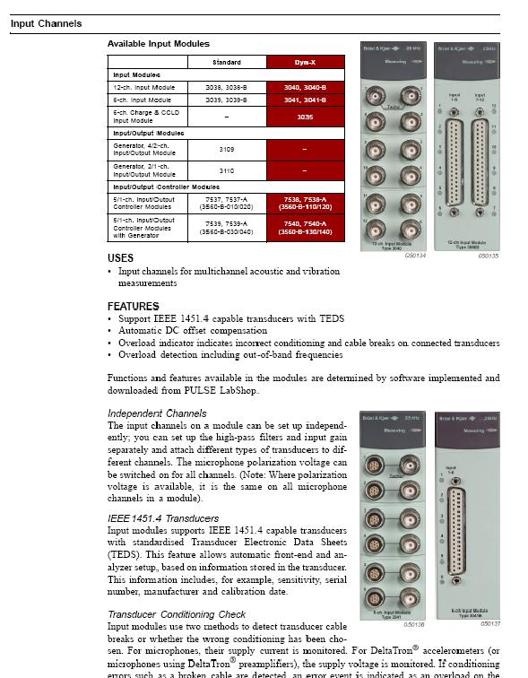
136 123

137 124

138 125

139 126

140 127

141 128

142 129

143 130

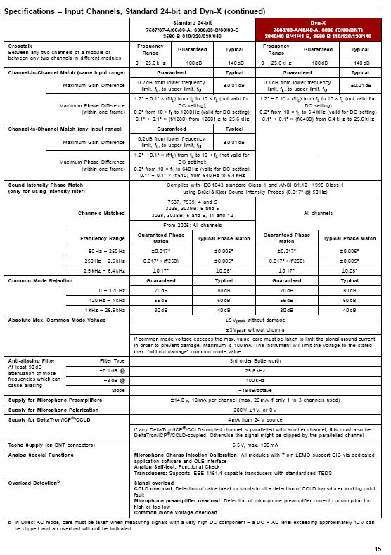
144 131

145 132

146 133

147 134

148 135

149 136

150 137

151 138

152 139

153 140

154 141

155 142

156 143

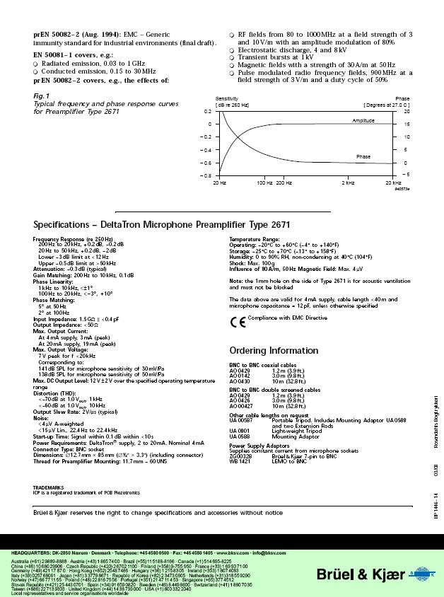
157 144

158 145

159 146

160 147

161 148

162 149

163 150

164 151

165 152

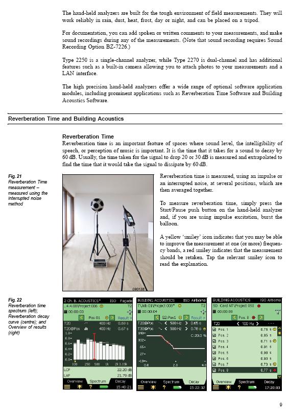
166 153

167 154

168 155

169 156

170 157

171 158

172 159

173 160

174 161

175 162

176 163

177 164

178 165

179 166

180 167

181 168

182 Reference C C. Time Domain Test Signal Inputs 169

183 Exhibit C1 60 db Steady Sinusoidal Test Signal with no Gaps Exhibit C2 60 db Steady Sinusoidal Test Signal with Gaps 170

184 Exhibit C3 65 db Steady Sinusoidal Test Signal with no Gaps Exhibit C4 65 db Steady Sinusoidal Test Signal with Gaps 171

185 Exhibit C5 70 db Steady Sinusoidal Test Signal with no Gaps Exhibit C6 70 db Steady Sinusoidal Test Signal with Gaps 172

186 Exhibit C7 73 db Steady Sinusoidal Test Signal with no Gaps Exhibit C8 73 db Steady Sinusoidal Test Signal with Gaps 173

187 Exhibit C9 80 db Steady Sinusoidal Test Signal with no Gaps Exhibit C10 80 db Steady Sinusoidal Test Signal with Gaps 174

188 Exhibit C11 85 db Steady Sinusoidal Test Signal with no Gaps Exhibit C12 85 db Steady Sinusoidal Test Signal with Gaps 175

189 Exhibit C13 90 db Steady Sinusoidal Test Signal with no Gaps Exhibit C14 90 db Steady Sinusoidal Test Signal with Gaps 176

190 Exhibit C15 94 db Steady Sinusoidal Test Signal with no Gaps Exhibit C16 94 db Steady Sinusoidal Test Signal with Gaps 177