O Behnam Bastani, 2005

Transcription

1 ANALYSIS OF COLOUR DISPLAY CHARACTERISTICS Behnam Bastani B.Sc Computing Science, Simon Fraser University, 2003 THESIS SUBMITTED IN PARTIAL FULFILLMENT OF THE REQUIREMENTS FOR THE DEGREE OF MASTER OF SCIENCE In the School of Computing Science O Behnam Bastani, 2005 SIMON FRASER UNIVERSITY Spring 2005 All rights reserved. This work may not be reproduced in whole or in part, by photocopy or other means, without permission of the author.

2 APPROVAL Name: Degree: Title of Thesis: Behnam Bastani Master of Science ANALYSIS OF COLOUR DISPLAY CHARACTERISTICS Examining Committee: Chair: Dr. Greg Mori Assistant Professor of Computing Science Dr. Brian Funt Senior Supervisor Professor of Computing Science Dr. Ghassan Hamarneh Supervisor Assistant Professor of Computing Science Dr. Tim Lee Internal Examiner Adjunct Professor of Computing Science Simon Fraser University Date DefendedJApproved:

3 SIMON FRASER UNIVERSITY PARTIAL COPYRIGHT LICENCE The author, whose copyright is declared on the title page of this work, has granted to Simon Fraser University the right to lend this thesis, project or extended essay to users of the Simon Fraser University Library, and to make partial or single copies only for such users or in response to a request from the library of any other university, or other educational institution, on its own behalf or for one of its users. The author has further granted permission to Simon Fraser University to keep or make a digital copy for use in its circulating collection. The author has further agreed that permission for multiple copying of this work for scholarly purposes may be granted by either the author or the Dean of Graduate Studies. It is understood that copying or publication of this work for financial gain shall not be allowed without the author's written permission.\ Permission for public performance, or limited permission for private scholarly use, of any multimedia materials forming part of this work, may have been granted by the author. This information may be found on the separately catalogued multimedia material and in the signed Partial Copyright Licence. The original Partial Copynght Licence attesting to these terms, and signed by this author, may be found in the original bound copy of this work, retained in the Simon Fraser University Archive. W. A. C. Bennett Library Simon Fraser University Bumaby, BC, Canada

4 ABSTRACT Predicting colours across multiple display devices requires implementation of device characterization, gamut mapping, and perceptual models. This thesis studies characteristics of CRT, LCD monitors and projectors. It compares existing models and introduces a new model that improves existing calibration algorithms. Gamut mapping assigns a mapping between two different colour spaces. Previously, the focus of gamut mapping has been between monitor and printer, which have relatively different gamut shape. Implementation and result of existing models are compared and a new model is introduced that its output images are as good as the best available models but runs in less time. DLP projectors with a different technology require a more complex calibration algorithm. A new approach for calibrating DLP projectors is introduced with a significantly better performance on predicting RGB data given tristimulus values. At the end, a new calibration method, using Support Vector Regression is introduced.

5 DEDICATION I dedicate this work to my awesome parents: Bijan Bastani and Mahnaz Gheibi for their time and support.

6 ACKNOWLEDGEMENTS I would like to thank Brian Funt for his support and guidance in this thesis and Ghassan Hamarneh for supervising me. My great friends, Roozbeh Ghaffari and Bill Cressman, are my great friends that helped me a lot. At last, I would like to thank my parents Bijan and Mahnaz for their constant support throughout my school time.

7 TABLE OF CONTENTS.. Approval... n... Abstract Dedication... iv Acknowledgements... v Table of Contents... vi... List of Figures... v~n List of Tables... xii List of Abbreviations... xiv Chapter 1: Introduction... 1 Chapter 2: Display Calibration... 5 Calibration Introduction... 5 Data Collection... 7 Device Characteristics Implementation Details D LUT Model Linear Model Masking Model Calibration Results Summary of the Calibration Study 29 Chapter 3: Optimal Device Calibration Introduction -34 CIELAB Weighted Least Squares (LabLS) 35 AE Minimization (DEM) 36 Measurement Charactenstics 36 Results -36 Summary of Optimal Device Calibration 38 Chapter 4: Gamut Mapping for Electronic Displays Gamut Mapping Introduction Characteristics of LCD and CRT Display Gamut Gamut Shape Predicting Out of Gamut Using Convex-Hull Algorithm to Predict Gamut Boundary Known Device-dependant GMAs... 46

8 Methods of Mapping Direction of Mapping Results of Device-based GMAs Clipping Implementation Non-linear Compression Mapping, Implementation Combination of Linear Transformation and Clipping Content Based Gamut Mapping Gamut Mapping to Preserve Spatial Luminance Variations: Bala [7] Space Sensitive Colour Gamut Mapping: Kimmel Summary of Gamut Mapping Chapter 5: DLP Projector DLP Projector Characteristic DLP Technology. Introduction Calibrating DLP Projectors Linear Model for DLP Projector Number of Channels Required Wyble's Model for DLP Projector Calibration Modified Wyble Method Masking Model DLP Calibration Results Summary of DLP Calibration DLP Projector Gamut Chapter 6: Lcd Projector Versus DLP Projector Temporal Stability Spatial Non-Uniformity [42] Chapter 7: Device Calibration via Support Vector Regression Introduction Applying SVR to Calibration Problem Results Chapter 8: Conclusion Chapter 9: Contribution Summary Reference List vii

9 LIST OF FIGURES Figure 2-1 : Percentage of the steady state luminance for white on the vertical axis versus the number of seconds since black was displayed on the horizontal axis....9 Figure 2-2: Measurement Error (Log scale) versus integration time in milliseconds measured for four greys on CRTl Figure 2-3: Channel Interaction. The horizontal axis represents the input value v ranging from 0 to 255 and the vertical axis represents the value of the channel interaction metric, CICOLOR(v,a,b). The black line shows a=b=255 and dashed lines show a=o,b=255 and a=255,b= Figure 2-4 Figure 2-5 Figure 2-6 Figure 2-7 Figure 2-8 Figure 2-9 Chromaticity shift shown as intensity is increased plotted in xy space with x=x/(x+y+z) on the horizontal axis and y=y/(x+y+z) on the vertical axis. When there is no chromaticity shift, all the dots of one colour lie on top of one another and therefore appear as a single dot Luminance curves for red, green, and blue phosphor input (Horizontal axis: R, G or B value. Vertical axis: L from CIELAB) Smoothing correction for non-monotonicity in the Z-response curve of the B channel for PR1. The vertical axis is the Z value reading and horizontal axis represents the digital counts for blue from 0 to Mapping Error versus Training Data Size Backward Error distribution for each characterization model on each device. AE error value is shown on the horizontal axis and histogram counts are shown on the vertical axis Comparison of Outliers for the Backward model. Vertical axis and horizontal axes represent Y./(X+Y+Z) and X./(X+Y+Z) respectively. The AE error is plotted according to the legend of grey scales. The circular points represent outliers with AE greater than 1.5 times the average error. The majority of the high outlier errors for LUT model occur near the gamut boundaries.. The outliers for Linear Model are quite negligible compared to the other two models Figure 2-10 Linearization failure for the black channel on PR Figure 4-1 Gamut shape of Displays in XYZ space Figure 4-2 Gamut shape of displays in L*a*b* space viii

10 Figure 4-3 Figure 4-4 Figure 4-5 Figure 4-6 Figure 4-7 Figure 4-8 Figure 4-9 Figure 4-10 Figure Figure 4-12 Figure 4-13 Figure 4-14 Figure 4-15 Gamut clipping and compression along a given direction. Target represent Target Gamut boundary and Source is the source (original) gamut boundary [ Directions for gamut-mapping Straight Clipping between source gamut (CRTI) and target gamut (LCD 1) at hue degrees Node Clipping between source gamut (CRTI) and target gamut (LCD 1 ) at hue degrees Cusp Clipping between source gamut (CRTl) and target gamut (LCD]) at hue ~10-20 degrees Choosing pivots in CIELAB space (A common colour name) Scatter of colours in a hue slice. The cusp (colour with maximum chroma) is the point with largest chroma value. Horizontal and vertical axis represent chroma and lightness...., Straight Clipping Result between source gamut (CRTl) and target gamut (LCD 1 ) Transformation applied before clipping. Result is between source gamut (CRT 1) and target gamut (LCD 1 ) Image gamut in CIELAB when its RGB channels are restricted to [50,150] range. Blue is the original gamut and red is the projected gamut General structure of Luminance-Preserving Gamut Mapping, Adapted from [7] A sample scene image that Bala's model does not improve the quality of output image over the Straight-clipping Comparison between Straight Clipping and Bala's model. Mapping is between source gamut (CRTI) and target gamut (LCD1) Figure 4-16 Result from Kimmel model with large alpha value only Figure 4-17 Result from Kimmel model with small alpha value only Figure Kimmel Result I: Kimmel model can recover clouds in the sky Figure 4-19 Kimmel Result 11: Flower Figure 4-20 Kimmel Result 111: Figure 4-21 Kimmel Result IV: From Louvre Museum Figure 5-1 Channel Interaction for DLP projector. The horizontal axis represents the input value v ranging from 0 to 255 and the vertical axis represents the value of the channel interaction metric, CIcoLoR(v,a,b). The black line shows a=b=255 and dark and light dashed lines show a=o,b=255

11 Figure 5-2 Figure 5-3 Figure 5-4 Figure 5-5 Figure 5-6 Figure 5-7 Figure 5-8 Figure 5-9 Figure 5-10 Figure 5-11 Figure 5-12 Figure 5-13 Figure 5-14 Figure 6-1 and a=255,b=0 respectively. For instance, on Green Interaction, light grey represents CI when R=255,B=O and G ramps from Chromaticity shift for DLP projectors shown as intensity is increased plotted in xy space with x=xl(x+y+z) on the horizontal axis and y=y/(x+y+z) on the vertical axis. When there is no chromaticity shift, all the dots of one colour lie on top of one another and therefore appear as a single dot. R,G,B,C,M,Y,W represent ramps of Red, Green, Blue, Cyan, Magenta, Yellow and White (~=g=b) Linear Model Result on dlp-toshiba projector. R and G are chromaticity channels represents r/(r+g+g) and g/(r+g+b respectively. The vertical axes represents error in AE White LUT for dlp-toshiba. All three LUTs have similar shape The LUTs for the four channel of Wyble's model Wyble Prediction Error in r/(r+g+b) and g/(r+g+b). The vertical axis represents AE94 error. Colours in the plot roughly represent their corresponding colours in RGB space Wyble Modified Prediction Error in r/(r+g+b) and g/(r+g+b). The vertical axis represent AE94 error. Colours in the plot roughly represent their corresponding colours in RGB space Masking Model Error in r/(r+g+b) and g/(r+g+b). The vertical axis represent AE94 error. Colours in the plot roughly represent their corresponding colours in RGB space Distribution of Forward and backward error for Wyble Model. Left and right columns represent the forward and backward error distributions respectively. Top and bottom rows represent the dlp-toshiba and dlp- Infocus displays Distribution of Forward and backward error for the Masking Model Left and right columns represent the forward and backward error distributions respectively. Top and bottom rows represent the dlp- Toshiba and dlp-infocus displays Gamut shape of dlp-infocus Gamut of dlp-toshiba...i03 dlp-toshiba gamut in CIELAB colour space Ramps of Red and Blue on the gamut when the other two channels are set to maximum Temporal Stability for 2 LCD and 2 DLP projectors. In the first 3 columns, changes in R, G and B channels are shown. Horizontal Access represents x/(x+y+z) and y/(x+y+z). Vertical access represents the data measurements

12 Figure Figure 6-4 Figure 7-1 Figure 7-2 The 9 points of screen measured to verify Spatial Non-Uniformity. 'C', 'R', 'L', 'T' and 'B' stand for Centre, Right, Left, Top and bottom comers. RB, LB are Right-Bottom and LeftBottom locations Spatial Non-Uniformity. The first column shows white measurements at 9 different locations on the screen for each display. Second column represents intensity (X+Y+Z) of white at each location. 'C', 'R', 'L', 'T' and 'B' stand for Centre, Right, Left, Top and bottom comers. RB, LB, RT and LT are Right-Bottom, LefLBottom, Right-Top and Left - Top locations SVR Error Insensitive Case. Data points outside the error range are ignored SVR Classification. SVR computes the closest point in convex hull of the data from each class

13 LIST OF TABLES Table 2-1 : Table 2-2 Table 2-3 Table 2-4 Table 2-5 Table 3-1 Table 4-1 : Table 4-2 Table 4-3 Table 4-4 Table 5-1 Table 5-2 Table 5-3 Table 5-4 Table 6-1 Table 6-2 Device Summary Forward mapping error: AE Mean (y ), standard deviation (o), and maximum Backward Error AE Mean (y), standard deviation (o), and maximum Percent Increase in Forward AE Error Due to Monotonicity Correction using Linear Model Experimental cpu time and storage space relative to the time and space used by the Linear Model Calibration Error in CIELAB AE Clipping comparison in AECIECAMO colours were used CRT I (source gamut) and LCD1 (target gamut) Effect of non-linear compression on gamut mapping between source gamut (CRT1) and target gamut (LCD]). This data is based on 1000 measured colour for each gamut. The change in gamut mapped colours is measured in AE...58 Difference between colours after TS-clipping is applied and before that. This data is based on 1000 measured colour for each gamut. The change in gamut mapped colours is measured in AE Comparing CPU time for Kimmel model under different resolution level. Data is the average CPU time for the model to converge on 600x800 image DLP projectors used in this thesis Scores for bases of PCA applied to each space. Scores are Residual Variance of each principal component. The scores can be used as an indication for the number bases required to sufficiently describe a space Forward Calibration Error in AE94 for DLP projectors based on 2277 points Backward Error in AE Projector names used Error caused by spatial non-uniformity for projectors xii

14 Table 7-1 Table 7-2 Four most common choices for Kernel function. d is the parameter to be set Performance of SVR for Calibrating 9 displays. Error is measured in... AEg xiii

15 LIST OF ABBREVIATIONS Delta E is a measurement of distance in CIELABg4 space. A value of one indicates a just noticeable difference in colour. Changes in CIECAM02 colour space. A value of one does not necessarily represent one noticeable change. CRT CMYK Cathode Ray Tube, a traditional type of display monitor which works by scanning a cathode ray from the back of the monitor across phosphors on the back side of the display screen Cyan, Magenta, Yellow, Black. In some cases, K is used to represent the grey axis. International Commission On Illumination L a* b* colour space. This is a perceptually uniform colour space, where a unit of distance anywhere in the space is intended to represent the same amount of perceptual difference. DLP GMA GOG LCD LUT OOG PCA RGB SVR Digital Light Processing, a new generation of projector technology designed by Texas Instruments. Gamut Mapping Algorithm, an algorithm for mapping between different gamuts Gain-Offset-Gamma, a term for a linear characterization model that assumes that the shape of the output curves is exponential, or "gamma" shaped. Liquid Crystal Display. A digital flat-panel monitor. Look Up Table Out of Gamut. This term refers to a colour that can be produced on one device, but is outside the gamut of the target device. Principal Component Analysis Red, Green and Blue. These are the colours of the phosphors, or primaries, in both LCD and CRT displays Support Vector Regression. xiv

16 UCR XYZ Under-colour removal. A technique used in printing, in which an appropriate amount of black ink is used to replace overlapping quantities of magenta, cyan, and yellow in dark areas. Used to refer to the CIE XYZ tristimulus space, where X and Z represent chroma and Y represents luminance.

17 CHAPTER 1: INTRODUCTION Accurate colour management across multiple displays is an important problem. Users are increasingly relying on digital displays for creating, viewing and presenting colour media. Users with multi-panel displays would like to see colour consistency across the displays, while conference speakers would like an accurate prediction of what their slides will look like before they enter the auditorium. To be able to predict colours across multiple electronic displays, implementation of several concepts, including device characterization, gamut mapping, and perceptual models is required. This thesis starts with studying characteristics of CRT and LCD monitors and projectors. Collecting data accurately is another important factor and some devices such as CRT monitors tend to take a longer time to stabilize their tristimulus output. Later on, several characterization models for LCD and CRT displays are studied. Device characterization is establishing a mapping from digital input values di (i=r,g,b) to tristimulus values such as XYZ. It is desired for a characterization model to be fast, use a small amount of data and allow for backward conversion from tristimulus values to di. Models need to be fast for real time application, i.e. previewing. Requiring small data size, makes it easy to combine multiple devices' characterization data into one and have it portable. Backward mapping is needed when the user wants to know what digital input values (di) are needed to have desired tristimulus values.

18 Three well-known characterization models are implemented in this thesis that support forward and backward mapping. The three models are 3D Look Up Table (LUT), Masking Model and Linear Model. The 3D LUT model [l] holds two 3 dimensional tables, one from forward mapping and one for backward mapping. The Masking Model was introduced by Tamura et. al. [2]. This model applies the concept of Under Colour Removal (UCR) to mask inputs from 3-dimensional RGB space to 7-dimensional RGBCMYK space, then linearizes the inputs and combines them with a technique similar to that used by the Linear Model. The term Linear Model refers to the group of models (GOG [3], S-Curve [2], and Polynomial [4] model) that estimate tristimulus response as a linear combination of pure phosphor outputs. These models each start by linearizing the digital input response curves with a specific nonlinear fbnction from which they draw their names. The Linear Model has been widely used for CRT monitors but has been criticized for its assumption of channel independence [2]. Channel independency is certainly an issue for LCD monitors from an industry point of view. In this thesis, we will study whether this characteristic exists when the end-user receives the displays. We will show a simple extension to the Linear Model (Linear+) that guarantees correct mapping of an important colour (e.g. white) without adding significant errors to other colours. This is simple substitution for gamut mapping which is discussed next. The gamut is the range of colours that a given device can produce. For a display, the colour gamut is the set of colours that the display can produce. For an image, the colour gamut is simply the set of all the colours found in it. In this thesis the gamut of several displays are studied, including gamut boundary and gamut shape. A method for

19 explaining the gamut boundary is also explained which takes advantage of the displays gamut shape. Gamut mapping is an important problem in colour management, and has been one of the most active areas of research in the Colour Imaging Conference series. The optimal gamut mapping approach for a given case depends on input and output device gamuts, image content, user intent and preference. Two major types of gamut mapping algorithms, display based and content based, are studied in this thesis. Display based gamut mapping algorithms are image independent and do not try to preserve the image content. This type of gamut mapping algorithm is normally fast since most of the work can be done before hand (such as defining the mapping) and the algorithm does not change based on image content. Several display based gamut mapping methods are implemented in this thesis including Cusp Clipping [5], Node clipping [6], Straight Clipping [5] and Rotation -based clipping. Content-based Gamut mapping algorithms try to preserve perceptual features of an image by redefining the mapping based on a pixel's neighbouring colours. In general, algorithms in this category include a refinement step after a device-based mapping is applied. Two methods in this category are studied in this thesis. The work by Balasubramanian [7] intends to reduce and adjust the trade-off between luminance and chrominance preservation by incorporating the pixel neighbourhood into the mapping. Kimmel [8] introduces a different approach for content-based gamut mapping. Kimmel's method refines the mapped pixels using information related to Retinex. This method is also linked to recent measures that attempt to combine spectral and spatial perceptual measures. Kimmel shows that if the target device gamut is convex, the gamut mapping

20 problem leads to a quadratic programming formulation, which is guaranteed to have a unique solution. The last part of this thesis studies the DLP (Digital Light Processing) projector technology. DLP projectors beside Red, Green and Blue components, include a fourth component, White, for enhancing subjective display quality. The Linear Model, using a 3x3 matrix, cannot predict the tristimulus values of DLP projectors accurately because of the fourth component [9]. In this thesis, a number of calibration methods are studied for DLP projectors and a model similar to the Masking Model [2] is shown to perform the best. The Gamut of DLP projector is also studied briefly and is shown that the gamut is not necessarily convex.

21 2.1 Calibration Introduction CHAPTER 2: DISPLAY CALIBRATION Accurate colour management across multiple displays is an important problem. Users are increasingly relying on digital displays for creating, viewing and presenting colour imagery. Users with multi-panel displays would like to see colour consistency across the displays, while conference speakers would like an accurate prediction of what their slides will look like before they enter the auditorium. Of course, displays will have been characterized and calibrated by the manufacturer; nonetheless the end user may well wish to verify and improve upon the calibration. We present a study of techniques for end-user calibration of CRT and LCD displays. Predicting colours across multiple display devices requires implementation of several concepts such as device characterization, gamut mapping, and perceptual models. The focus of this thesis is device characterization by an end user, with the goal of selecting an appropriate model for mapping digital input values di (i=r,g,b) to tristimulus values such as XYZ. A good characterization model should be fast, use a small amount of data, and allow for backward mapping from tristimulus to d,. Backward mapping is useful when user is interested in finding RGB values that result in a given XYZ values. For example in previewing, a user is interested in previewing on a one display an image as it will appear on a second display. A backward mapping is required for the preview display.

22 There are a several well-known characterization models that support both forward and backward mapping, three of which were implemented in this experiment: a 3D Lookup Table (LUT), a Linear Model and a Masking Model. The LUT method [I] uses a 3-dimensional table to associate a tristimulus triplet with every RGB combination and vice versa. This method is simple to understand but difficult and cumbersome to implement. The term Linear Model refers to the group of models (GOG [3], S-Curve[2], and Polynomial[4] model) that estimate tristimulus response as a linear combination of primary colour outputs. These models each start by linearizing the digital input response curves with a specific nonlinear function from which they draw their names. The Linear Model has been widely used for CRT monitors but has been criticized for its assumption of channel independence [2]. We will show a simple extension to the Linear Model (Linear+) that guarantees correct mapping of an important colour (e.g., white) without adding significant errors to other colours. The third model implemented in this study is the Masking Model introduced by Tamura, Tsumura and Miyake in 2002 [2]. This model applies the concept of Under Colour Removal (UCR) to mask inputs fiom 3-dimensional RGB space to 7-dimensional RGBCMYK space. It then linearizes the inputs and combines them with a technique similar to that used by the Linear Model. This thesis will discuss the implementation, benefits and pitfalls of each method with respect to use on CRT and LCD display devices. In general, prediction errors will be quantified terms of AE, as measured in 1994 CIE La*b* colour space. The first section of the thesis deals with data collection. The next section reviews the characteristics of the

23 devices used in the study. Section Three discusses implementation details and considerations for each of the characterization models. Section Four reviews the results of the study. 2.2 Data Collection All data used in this study was collected using a Photo Research Spectrascan 650 Spectroradiometer in a dark room with the spectroradiometer at a fixed distance, perpendicular to the center of the display surface. Spectroradiometer is an instrument for determining the radiant energy distribution in a spectrum combining the functions of a spectrometer with those of a radiometer. Before beginning each test, the monitor settings were re-set to the factory default, and the brightness was adjusted using a grey-scale calibration pattern until all shades of grey were visible. The data collection was performed automatically in large, randomized test suites. We found that it is important to test the repeatability of the spectroradiometer with respect to each monitor, and ensure that the test plan is sufficient to smooth out the measurement errors. As a result, each RGB sample used in this study was derived from of a total of 25 measurements taken in 5 randomly scheduled bursts of 5 measurements each. This technique served to average out both long- and short-term variation. The size and quantity of bursts were determined through empirical study. An issue that arises when using an automated data collection system is phosphor stabilization time. Figure 2-1 shows the percentage of steady-state luminance for white versus the number of seconds since a colour change from black. "Luminance," as used here, is the L value in CIELABw space. Note that the LCD-based devices reach steady

24 state within less than 5 seconds, while the CRT devices take longer. However, the amount of time required for the CRT devices (up to 10 seconds) was somewhat surprising. The spike on CRT2 that occurs right after the colour change is unexpected as well. In practice, we found that using a delay of 2500 ms between the display of a colour and the start of measurement gave acceptable results.

25 Figure 2-1: Percentage of the steady state luminance for white on the vertical axis versus the number of seconds since black was displayed on the horizontal axis. CRTl

26 An additional important setting related to data consistency is spectroradiometer integration time. Integration time is the number of milliseconds the spectroradiometer's shutter remains open during a measurement. The integration time needs to be adjusted as a hction of the incoming signal. In general, CRT monitors require a longer integration time because the display flashes with each beam scan. Figure 2-2 shows the result of an integration time test on CRT1. Observe that shorter integration times result in more unstable measurements. The monitor refresh rate used in this experiment is 75 Hz, which equates to 13.3 ms per scan. Therefore, any integration time t will experience either Lt or rtl13.31 scans depending on when the measurement window starts. For example, if the integration time is 1 OOms, then measurements will either experience seven or eight scans, leading to high variation. Conversely, a time of 400 ms will almost always lead to 30 scans ( 400 I = ).

27 Figure 2-2: Measurement Error (Log scale) versus integration time in milliseconds measured for four greys on CRTl Integration Time The measurements in this study were taken with a default integration time of 400ms, which was doubled whenever a "low light" error was reported by the spectroradiometer and halved when a "too much light" error was reported. Although this technique resulted in acceptable error levels, an improvement would be to ensure that all integration times are exact multiples of 13.3, so each measurement gets the same number of scans. Three suites of data were collected for each monitor: a 10x10x10 grid of evenly spaced RGB values covering the entire 3D space, a similar 8x8~8 grid used for testing and verification, and a "1 01x7" data set made up of 101 evenly spaced measurements for each RGB and CMYK channel with the other inputs set to zero.

28 2.3 Device Characteristics Seven devices were tested: two CRT monitors, three LCD monitors, and two LCD projectors. A summary of these devices is given in Table 2-1. One important issue in characterizing a display is whether each channel's response is independent of the other channels. In this study, channel interaction is calculated as follows. Table 2-1: Device Summary Name Description Interaction Mean Interaction Max CRTI Samsung Syncmaster 900NF 2.1% 9.4% CRT2 NEC Accusync 95F 1.5% 4.9% LCD1 IBM % 0.4% LCD2 NEC 1700V 2.2% 4.1% LCD3 Samsung 171 N 1.2% 2.7% PRI Proxima LCD Desktop Projector % 0.5% PR2 Proxima LCD Ultralight LX 0.4% 0.7% In this equation, v represents the input value for the channel in question, a and b are constant values for the other two channels, and L(r,g,b) represents the measured luminance for a given digital input. The equations for CIGREEN and CIBLUE are similar. This equation measures how much the luminance of a primary changes when the other two channels are on. The overall interaction error for each device (Table 2-1) was calculated as

29 where N is the averaging factor = (XS+ 1 )*3. From end-user point of view, three of the five LCD devices showed almost no channel interaction; however, both CRT monitors exhibited significant channel interaction (Figure 2-3). The interaction on the CRT monitors was generally subtractive (leading to lower luminance) while on the LCD monitors it was either additive or negligible.

30 Figure 2-3: Channel Interaction. The horizontal axis represents the input value v ranging from 0 to 255 and the vertical axis represents the value of the channel interaction metric, CICOLOR(v,a,b). The black Line shows a=b=255 and dashed lines show a=o,b=255 and Red Green Blue

31 Another potential issue with LCD monitors is a possible chromaticity shift of the primary colours. Figure 2-4 shows the chromaticity coordinates for each of the primary colours (RGB), as well as the combined colours (CMYK), after dark correction, plotted at 10 luminance settings per colour. It was observed that all devices have stable RGB chromaticity; however, all the LCD devices exhibited significant chromaticity shifts in the combined (secondary) colours. The cause of chromaticity shift is explained in detailed by Marcu [55]. The presence of a chromaticity shift in the secondary colours (CMYK) will cause problems with the Masking Model since it uses the combined colours (CMYK) as primaries. The problem arises in the response-curve linearization step, where it will not be possible to find a linearization function that makes all three curves into lines. As a result, the linearization will be poor which will then lead to erroneous output estimates.

32 Figure 2-4 Chromaticity shift shown as intensity is increased plotted in xy space with x=x/(x+y+z) on the horizontal axis and y=y/(x+y+z) on the vertical axis. When there is no chromaticity shift, all the dots of one colour lie on top of one another and therefore appear as a single dot. CRTl

33 2.4 Implementation Details All characterization methods start with black-level correction in which the measured XYZ value of black (minimum output) for the device is subtracted fiom the measured tristimulus value of each colour. This ensures that all devices have a common black point of (0,0,0) in XYZ space. Fairchild et. al. discuss the importance of this step [50]. The remaining steps for each characterization differ based on the method and are described below D LUT Model The 3D LUT method was implemented with the intention of provic ding a standarc against which to evaluate the other two models [I]. It is expensive both in time and space (-10 MB for the lookup table) and is not well suited for reverse mapping. To create the forward lookup table, the 1 Ox 1 Ox 10 training data is interpolated using 3D linear interpolation to fill a 52x52~52 lookup table indexed by RGB values spaced 5 units apart. At look-up time, 3D spline interpolation is used to look up intermediate values. Inverting the lookup to index by XYZ requires interpolation of a sparse 3D data set, which is non-trivial and an independent area of research [49]. The reverse lookup was performed via tetrahedral interpolation into the original 10x10x10 data set. Tetrahedral interpolation was chosen over a number of other methods primarily for its speed and its ability to handle sparse, irregularly spaced data Linear Model The Linear Model is a two-stage characterization process. In the first step, the raw inputs di (i=l, 2, 3 for R, G, B) are linearized using a function Ci(di) fitted for each

34 channel. Linear regression is then used to determine the slope Mij between each linearized input Ci(di) and the respective XYZ outputs where j=(l, 2, 3) for (X, Y, Z). The second stage applies matrix M to calculate estimated XYZ values. The LUT is calculated as follows. The 10 measured response values for the ith input channel are interpolated to obtain three output vectors X(di), Y(di) and Z(di) in 256- dimensional space. Principal component analysis is then used to find the single vector Ci(di) that best approximates all three vectors. The following equation calculates Ci(di) where PCAi represents the weighting vector obtained from principal component analysis for channel i In order to allow for backward mapping, two conditions are required: the linearization function must be monotonic and the matrix M must be invertible. Inversion is always possible because the input channels are linearly independent. However, the monotonicity requirement is a real problem with LCD displays where the response curves sometimes level out or even decline for high input values (Figure 2-5). It is therefore necessary to modify the linearization function to ensure monotonicity as shown in Figure

35 2-6. Note that this modification, although necessary for backward mapping, reduces the accuracy of the linearization and increases the error of the forward characterization. Figure 2-5 Luminance curves for red, green, and blue phosphor input (Horizontal axis: R, G or B value. Vertical axis: L from CIELAB) CRTI - Luminosity CRT2 - Luminosity rn f LCD1 - Luminosity LCD2 - Luminosity m LCD3 - Luminosity 300 r, 1 Projector1 -LCD - Luminosity I I Projector2-LCD - Luminosity I

36 Figure 2-6 Smoothing correction for non-monotonicity in the Zresponse curve of the B channel for PR1. The vertical axis is the Z value reading and horizontal axis represents the digital counts for blue from 0 to Before Smoothing After Smooth~ng Q) P When creating the lookup table, a decision must be made regarding the size of the training data set. Figure 2-7 shows the effect of training size on the forward mapping error measured in AE. In general, a larger training set is better, but the benefit tapers off after about 10 data points. For the results section of this thesis, a training data set with 101 points was used to ensure minimal error introduced by training data size.

37 Figure 2-7 Mapping Error versus Training Data Size Pebuv (LCD) - - AS Projector The primary criticism of the Linear Model is that it assumes channel independence. As we have seen above, this is not always a valid assumption - even for CRT monitors. When there is channel interaction, the predicted output XYZ value for colours that use more than one primary colour may not be accurate. Predicting white and grey values correctly is crucial in colour calibration [51]. For example, white is significant on computer-generated images such as presentation slides or charts where there are large regions of pure white with no ambient lighting expected. We observed that the Linear Model in general overestimates the luminance of white. There are several approaches to addressing this issue. One technique, WPPPLS, imposes a constraint so that the Linear Model emphasizes correct prediction of white [51]. A simple approach is to apply a diagonal transform to the slope matrix M based on the measured and predicted values of pure white. The following formula shows the conversion, where XMEASURED is the measured X value for white and XPRE~~CTED is the predicted X value for white using the original slope matrix,.

38 This modification to the slope matrix ensures that white is correct, but slightly shifts all of the other colours in a non-uniform manner, which could potentially increase the overall error. This model will be referred to as "Linear+" in this thesis, and is useful when displaying computer-generated images such as charts where white is a major colour. Note that a similar correction can be performed using predicted values in an alternate space, such as LMS cone sensitivity space. In our study, we found that using either XYZ or LMS intermediate space returns the nearly same average increase in forward error (*0.05 AE for all devices). Further improvement may be possible using a technique similar to that presented by Finlayson and Drew in [511, where a modified least-squares procedure is used to determine the matrix M. By constraining the prediction error for white to zero, a matrix can be selected that reduces overall error while ensuring an accurate white value. It is interesting to note that their approach achieved good results even without first linearizing the inputs Masking Model The Masking Model [2] attempts to avoid problems related to channel interaction with a technique similar to under colour removal in printing. The original digital input di

39 (i=1,2,3 for RGB) is converted to masked values mi (i=1,2,3,4,5,6,7 for RGBCMYK), and the masked values are combined in a manner similar to that for the Linear Model. The masking operation assigns values to three elements of m - the primary colour (index p), the secondary colour (index s), and the grey colour (index 7), and sets all of the remaining elements of m to zero, as follows. Primary color index p such that d, = max(d,, d,, d, ) Under color index k such that d, = min(d,, d,, d,) & k # p Secondary color index s = k + 3 Primary color m, = d, Secondary color m, = d,-,-, Gray (Under) color m, = d, Unused Color m,,~p,s,7, = 0 The result of these formulas is to set p to the index of the maximum primary colour (R, G, or B), and m, to the input value for that colour. It assigns s to the index of the mixed colour (C, M, or Y) that does not contain the minimum colour, and assigns m, to the median of the original values. Finally, it sets the grey (under colour) value m7 to the minimum of the three original inputs. For example, if the original inputs are RGB=(200,180,30), the primary colour will be red, with a value of 200. The secondary colour will be yellow (which does not contain blue) with a value of 180, and the grey (under) colour will have a value of 30. The masked input array becomes m=[200,0,0,180,0,0,30].

40 Once the inputs have been converted into masked values mi, a linearization function Ci(mi) for each input channel i is determined using the method described above for the Linear Model. The slope matrix Mij for each input channel i and output channel j is calculated as using PCA and linear regression, also as described for the Linear Model. Finally, let the vector Pi represent the column of matrix M that contains the X, Y, and Z slopes for input channel i. The transformation from masked input to XYZ output can then be written as follows: Here C,, C, and C7 represent the linearization functions for primary, secondary and black component. The mi values are the values corresponding to each basis (primary, secondary or black). The inverse mapping from XYZ to RGB is less obvious, and requires knowledge of the primary and secondary colour indices p and s. There is no way to know these values, so all six possible (p, s) combinations are tested (RM, RY, GC, GY, BC, BM) and any combination that satisfies the following conditions will yield the correct result.

41 2.5 Calibration Results We calculated values of forward error AEFwD, round trip error AETRIP, and backward error AEswD for 512 colours in an 8x8~8 evenly spaced grid of RGB inputs. For each colour, we find three vertices in CIE L*a*b* space: the measured value for the colour VM, the predicted value vp, and a round-trip value VRT. The round-trip value is found by mapping backward and forward again fiom vp. These points form a triangle with edges representing the forward, round-trip and backward error vectors. AEFWD is the distance from VM to vp, AETR~P is the distance fiom vp to VRT, and AEswD is the distance fiom VRT back to VM. With respect to forward or backward error, we see that the 3D LUT is the most accurate, followed by the Linear, Linear+ and Masking Models (Table 2-2, Table 2-3). Note, however, that the Linear and Masking Models all have a round-trip error of zero, while the 3D LUT has a non-zero round-trip error indicating an imperfect inversion. This is not surprising considering the rounding error inherent in the sparse 3D interpolation required to build the backward lookup table. The other interesting observation is that Lin+ improved average forward error for CRTl which has higher CI than CRT2. This data confirms that most of the error was due CI and a simple modification to the Linear Model improves the overall performance.

42 Table 2-2 Forward mapping error: AE Mean (p ), standard deviation (a), and maximum. I I LUT I Lin I Lin+ I Mask I p CRTI 0.8 CRT2 0.5 LCD max p 0 max p 0 max p 0 max Average ( ( Table 2-3 Backward Error AE Mean (p), standard deviation (a), and maximum. PRI I 12.3 PR Average A comparison of backward error distributions (Figure 2-8) shows that the Linear Model had the most compact distribution for each device, while the distribution for 3D LUT tended to have a number of high-error outliers. The cause of these outliers becomes

43 apparent when the error values are plotted by chromaticity (Figure 2-9). Observe that the largest errors for the 3D LUT are often on or near the gamut boundary. For the Linear Model, the highest errors are fairly well distributed across the chromaticity space for all devices except the projectors, which have a distinct problem in the blue region. This is most likely due to the non-monoticity exhibited by the projectors in the blue output curves (Figure 2-5). As mentioned in the implementation section, the monotonicity correction stage is a potential source of error for all devices. However, it appears to be adding very little error for devices that do not have a monotonicity problem (Table 2-4). The most notable increase in error was seen with the Projector 1, which also had the most trouble with non-monotonicity. Table 2-4 Percent Increase in Forward AE Error Due to Monotonicity Correction using Linear Model I Uncorrected I Corrected [ % increase CRTl I 2.4 I 2.4 I 0.0% Average I 2.2 I 2.2 I 2.3% The average error for the Linear+ model was nearly the same as that for the standard Linear Model. Recall that the goal of Linear+ is to guarantee that the predicted white is correct, at the possible expense of other colours predictions. The results in Table 2-2 and Table 2-3 show little increase in overall error, which means a "perfect" white can

44 be achieved without much degradation in other colours. Informal visual comparisons indicate that this model is often the best one to use for computer-generated graphics. The Masking Model was expected to out-perform the Linear Model whenever there was an issue with channel interaction. However, the model's best performance (on CRT2) is only slightly better than that of the Linear Model. The primary pitfall of this model is that it depends on constant-chromaticity "combined primaries" (CMYK). It is clear from Figure 2-4 that this assumption fails for the LCD monitors and projectors. The chromaticity shift causes the input the linearization step to fail. Figure 2-10 shows an example of an unsuccessful linearization for the black channel for PRl in the Masking Model. This explains why the performance of the Masking Model was better for the CRT monitors than any of the other devices- the CRTs do not have the shifting chromaticity problem. It is also interesting to note that on CRT2, the Linear+ algorithm introduced the largest amount of error, indicating that the interaction present on this monitor is not well suited for correction with non-uniform scaling. With respect to efficiency, the Linear Model is the best. The Linear Model is slightly faster than the Masking Model and nearly 20 times faster than the 3D LUT. The Linear Model also requires less than half the storage space of the Masking Model, and less than 11300th the storage space required for 3D LUT (Table 2-5).

45 Table 2-5 Experimental cpu time and storage space relative to the time and space used by the Linear Model Linear Masking 3D LUT Time 1.O Space 1.O Summary of the Calibration Study Several display characterization models were implemented in this thesis: a 3D LUT, a Linear Model, an extension to the Linear Model, and a Masking Model. These characterization models were each tested on seven devices: two CRT Monitors, three LCD monitors and two LCD projectors. The devices are characterized from and end user perspective in which the devices are treated as black boxes with no knowledge or control over their internal workings. In characterizing the devices, two issues that were of particular importance were phosphor stabilization time and spectroradiometer integration time (Figure 2-1, Figure 2-2). We found that the phosphor stabilization time on the CRT monitors can take up to 10 seconds. In practice, a delay time of 2500 ms between colour display and measurement resulted in acceptable error levels. With respect to integration time, we propose that measurements on CRT monitors be taken with integration times that are multiples of the display scan rate. In addition, we observed that a training set of 10 data points per axis was sufficient for an accurate Linear Model for each of our 7 displays. (Figure 2-7). Although recent thesiss have indicated that the Linear Model is not applicable to LCD panels [2], it worked well for the LCD display tested in this experiment. Furthermore, the channel interaction problem was more pronounced on the CRT monitors

46 than on several of the LCD displays. The fact that we did not find channel interaction with the LCD's we tested does not mean that it is not present in LCD panels themselves. We tested completed LCD displays which include electronics specifically designed to mitigate the effects of channel interaction. Nonetheless, from an end-user point of view, channel interaction did not pose a problem. The primary issue with the LCD displays was the fact that the response curves for the three input channels were dissimilar, leading to chromaticity shift of combined colours (CMYK). This problem affected the Masking Model but not the Linear Model. Despite these issues of linearization and channel interaction, all three models yielded a level of error that on average has a mean of less than 4 AE and a worst case less than 15 AE. The 3D LUT model was slightly more accurate than the other models, but it is too cumbersome for actual use. The Linear Model was the most efficient, with accuracy nearly as good as to the 3D LUT. The primary drawback of the Linear Model is that it can be adversely affected by channel interaction. A slight modification to the Linear Model is presented in the Linear+ model that uses a simple white-point correction technique to ensure correct prediction of white. Our results indicate the Linear+ model is able to guarantee white-point accuracy with minimal degradation for other colours.

47 Figure 2-8 Backward Error distribution for each characterization model on each device. AE error value is shown on the horizontal axis and histogram counts are shown on the vertical axis. Linear Model AEBACKWARD Masking Model AEBACWARD

48 Figure 2-9 Comparison of Outliers for the Backward model. Vertical axis and horizontd axes represent YJ(X+Y+Z) and M/(X+Y+Z) respectively. The AE error is plotted according to the legend of grey scales. The circular points represent outliers with AE greater than 1.5 times the average error. The majority of the high outlier errors for LUT model occur near the gamut boundaries.. The outliers for Linear Model are quite negligible compared to the other two models. 3D LUT Linear Model Masking Model

49 Figure 2-10 Linearization failure for the black channel on PR Linearized M Channel Input

50 CHAPTER 3: OPTIMAL DEVICE CALIBRATION 3.1 Introduction In this section, we try to study whether the traditional Device Calibration used for electronic display can be improved. As was explained earlier, a forward Linear Model is based on a 3-by-3 linear transformation matrix M mapping data from (linearized) RGB to XYZ. A typical approach for generating the matrix M is by applying least squares between linearized RGB and measured XYZ [511 or using principal component analysis (Section 2.4.2). Although these two methods for calculating M work well, they both suffer from the fact that they try to minimize error in XYZ space, which is perceptually non-uniform. In this chapter we propose two methods for calculating M which is based on more directly optimizing the error measure in CIELAB. The first approach (LabLS) extends the least-square model (ULS) by applying weights to the model. Weights represent importance of a colour in CIELAB space (the space that is important to us). The second method is based on optimizing the AE error directly using the Nelder- Mead simplex algorithm [56]. Unfortunately, the Nelder-Mead algorithm (not to be confused with the linear programming simplex algorithm) finds a local minimum and does not guarantee a globally optimal solution. However, by using the results of the LabLS method as the starting condition, we have found experimentally that it converges reliably to excellent solutions. This method will be referred to as DEM since it is based on a AEg4 minimization.

51 3.2 CIELAB Weighted Least Squares (LabLS) This method extends the standard least squares solution to a weighted least squares solution in which the weights are defined to be inversely proportional to the approximate size of the MacAdam colour discrimination ellipse that would surround each XYZ. The weights for the LabLS method are based on human sensitivity to colour differences as encapsulated in CIELAB AE. The idea is to evaluate the rate of change in L*a*b* as a hction of change in XYZ. The 3-dimensional change (AX, AY, AZ) represents a change in a volume, which can be formalized in Equation (9) as the cube root of the absolute value of the Jacobian determinant. For each measured XYZ, the corresponding weight is calculated and arranged along the diagonal of a matrix W. M is then calculated using equation (lo), where D is an 11x3 matrix containing normalized XYZ tristimulus values and N is an 11x3 matrix containing the linearized RGBs. This use of the Jacobian of L*a*b* is similar to that proposed by Balasubrarnanian [57] in the context of colour printer calibration and by Sharma and Trussell [58] in the context of colour scanners.

52 3.3 AE Minimization (DEM) Nedler-Mead simplex [56] search is a directed search method for multidimensional non-linear regression. This search can be used to optimize the 9 parameters in matrix M so that the calibration error is minimized. In this thesis we used the Matlab function fininserach to find the 9 values in matrix M, however any local-search algorithm can be used. The solution depends on the starting conditions. It is shown below that the Nedler-Mead simplex search outperforms other models when it starts with an initial solution found by LabLS. 3.4 Measurement Characteristics We used the measurements for the 7 displays mentioned in Table 2-1 that was originally used to compare Linear Model and Masking Model performance. Similarly, all three RGB channels are linearized respect to XYZ values. 3.5 Results The ULS, LabLS and DEM methods of computing the RGB-to-XYZ transformation matrix, M, were applied to the same 1000 measured colours as in Chapter 2. All these values are used after they are linearized and normalized with respect to the

53 white of the display. In each case, the resulting M is evaluated by using it to map the 1000 RGB inputs to XYZ and measuring the difference between the predicted and measured values. The difference is calculated in terms of the average AE94 error measures. Table 3-1 shows the performance of the three Linear Models in AE94. In the tables, 'mean,' 'std' and 'max' are the average error, standard deviation and maximum error over the 1000 test samples. The percentage improvement in error relative to unweighted least squares is labeled 'change'. None of the methods requires more that a few seconds of computer time to solve for M. Table 3-1 Calibration Error in CIELAB AEg4

54 Std ULS 1.44 LabLS DEM Mean I Change I 1 10% 1 15% I Max Std Mean Change % % Std I Mean I Change I 1 4% 1 5% I Max I Std Comparing Table 3-1 with Table 2-2 shows that there is no advantage between calculating the matrix M using Least Squares (ULS) or using coefficient of PCA (Section 2.4.2), and both LabLS and DEM have improvements over the old two methods. 3.6 Summary of Optimal Device Calibration The performance of a 3x3 linear colour calibration model can be improved by optimizing for the transformation matrix in spaces other than XYZ. One alternative (DEM) is to minimize directly in CIELAB space, but this involves nonlinear optimization. Another alternative (LabLS) is to optimize using weighted least squares regression in a CIELABweighted version of XYZ. Experiments in calibrating with 7 different displays show that both methods significantly reduce calibration errors as measured in terms of average and maximum AE94 error.

55 CHAPTER 4: GAMUT MAPPING FOR ELECTRONIC DISPLAYS 4.1 Gamut Mapping Introduction A gamut is the range of colours that can be formed by all combinations of a given set of light sources or colourants of a colour reproduction system. The human eye can perceive a wide gamut of colours within the full range of the visible spectrum, including detail in very bright light and deep shadows. Reflected light, ink impurities, and paper absorption, all limit a conventionally printed image colour gamut [I 11. Similar effect happen on monitors and projectors as each display can produce a limited range of colours. Similarly, we can define a gamut for an image, which is the set of all the colours found in it. In this thesis, we focus on the gamut of electronic display and more specifically on the CRT and LCD displays. In order to be able to preview one display's output on another display, we need to find a way to overcome the difference between gamuts of displays. The source gamut is the gamut of a display or an image that is desired to be mapped. The target gamut, on the other hand, is the gamut of the display that the image is intended to be viewed on. The Gamut Mapping Algorithm (GMA) try to find a mapping between the two gamuts. A GMA should allow for different rendering intents (e.g. accuracy, pleasant, retinex reproduction). Most GMAs are based on the assumption that the design of the optimal technique involves combination of image attributes such as contrast, luminance detail, vividness,

56 and smoothness. The followings are the general measurement factors and goals for a GMA identified by Jan Morovic [ 131 and MacDonald [ 151. Preserve the Grey Axis of the image for maximum luminance contrast. Minimize the hue shift. Most of the display-based GMAs are designed to preserve the hue angle by allowing changes in saturation or luminance. Increase in saturation is preferred. Even though the saturation might be limited after the gamuts are mapped, at least the available potential saturations should be used. There are two general gamut mapping algorithms [7]. The first category is solely device dependent, where gamut mapping is a fimction of input and output device gamut and the algorithm is independent of image content. The majority of gamut mapping algorithms fall in this category [13]. In this approach, the gamut mapping is a point-wise operation from an input point to an output point in an appropriate (usually perceptual) 3D colour space. One of the fundamental problems with such point-wise operation is that it does not take important spatial neighbourhood effects in an image into account. We refer to this type of GMA as device-based GMA. The second category of gamut mapping algorithms, content-based GMA, considers spatial characteristics in addition to colour characteristics of the image. Using these algorithms, two pixels of the same colour in an image can map to different colours in the output image, depending on the spatial characteristics in the neighbourhood of the pixels.

57 The majority of the study on GMAs is between monitors and printers that have a very different gamut shape. In this thesis, we specifically focus on gamut mapping between electronic displays. We show improvements that we can make to existing GMAs by considering common characteristics between gamut of electronic displays. This section starts by studying the properties of LCD and CRT gamuts. Methods for determining gamut boundary and finding OOG are explained. The next part starts with a detailed introduction to different types of device-based GMA. We introduce an algorithm for fitting most of the source gamut inside the target gamut before any devicebased mapping is applied to bring the remaining OOG colours inside gamut. This algorithms is based on the similar shape of the gamut of displays and tries to preserve the hue angle for each colour. At the end, performance of this new algorithm is compared to other existing algorithms, including some content-based GMAs that take longer CPU time. 4.2 Characteristics of LCD and CRT Display Gamut Gamut Shape Electronic displays such as LCD and CRT displays have an additive gamut compared to a printer's gamut which has a subtractive gamut. Additive means that their gamuts are created by adding lights; whereas for printers, the gamut is created by reducing reflectance light from the paper. In Color.org [14] website there is a visual comparison between CRT monitor gamut shape and a 4-ink inkjet printer. It is obvious that these two devices, monitor and printer, have different shape, one is quite convex and the other one has concavities in multiple places.

58 Out of 7 displays shown in Table 2-1 that we studied in this thesis, we observed that all of them have a convex shape gamut with very similar shape. In general, it is expected that these devices will have a convex gamut since their colour space is generated in an additive form by combining three different lights (R, G, B). Figure 4-1 and Figure 4-2 show 1500 colours measured inside each of these gamuts in XYZ and CIELAB colour space.

59 Figure 4-1 Gamut shape of Displays in XYZ space C RTI

60 Figure 4-2 Gamut shape of displays in L*a*b* space CRTl CRT'2,..'I.._... :.. _ joo-.." :.. *......: -P '._...I: a* L* a* L*

61 From these two figures we can see that all the devices that we tested have a convex gamut shape. In this thesis we try to take advantage of this property of display gamut for mapping colours and predicting the gamut boundary Predicting Out of Gamut Predicting the gamut boundary, and as a result finding OOGs, is quite challenging when a gamut is concave. However, as it was shown earlier, we can assume that LCD and CRT gamuts are convex. Knowing this property simplifies the prediction of the gamut boundary and finding OOGs. The simplest approach to calculate a convex surface is by finding the convex hull of the set of given points, in this case measured XYZ or L*a*b* values. The convex hull of a data set in n-dimensional space is defined as the smallest convex region that contains the data set [211. In our case, since we are working with a three-dimensional data-set (XYZ or L*a*b*), the facets that make up the convex hull are triangles. References [22] and [23] have detailed information on the convex-hull algorithm. In this thesis we use a convex-hull implementation provided by Matlab Using Convex-Hull Algorithm to Predict Gamut Boundary We can tessellate the surface of convex hull into triangles. Each triangle represents a plane in 3D colour space. A plane in a 3-dimensional space is represented by ax + by + cz - K = 0'. Now if we substitute a point (Xo, YO, Zo) into the formula, three things can happen. The equation axo + byo + czo - K can equal to zero meaning the ' Similar situation applies to L*a*b* values in CIELAB colour space.

62 point is on the plane. If the point is outside the plane, then the equation will be less or greater than zero, depending on which side of the plane the point is. This simple idea can be used to find whether a point, PA is outside the hull. If the sign of one of the plane equations for convex hull boundary evaluated at a point, PA, is different than the sign of the same plane evaluated on a point inside gamut, Pf, then the PA is out of gamut. If we have N triangles, and thus N plane equations, the time complexity of this algorithm to find out if a colour is inlout of gamut is O(N). In general for the displays in this thesis, we only needed under 250 triangles to represent the gamut surface. This means that the algorithm can be quite fast. 4.3 Known Device-dependant GMAs Device-dependant GMAs clip out OOG on or inside the target gamut boundary. Their difference lies in how and where these points are clipped and whether inside-gamut colours are changed. Sometimes, there is more than one name refemng to the same GMA and for clarity, we use the terms introduced by CIE [14]. In this section, we start by looking at different methods of mapping. We introduce an extension to the clipping algorithms and in the next section, we compare the performance of all the device-based mapping. Evaluating GMA performance requires visual comparison and for this thesis we did not run a human study. The models were evaluated by the graduate student, Behnam Bastani. In most cases the difference is quite noticeable. Some of the images are provided later in this section for the reader.

63 4.3.1 Methods of Mapping There are two general types of mapping in device-dependant GMA. The first method, Gamut Clipping, changes only the colours outside of the gamut either after or before lightness compression [5]. There are several methods for compressing lightness. A lightness compression method introduced by Montag and Fairchild, [24], compresses the source gamut in the lower lightness part with a higher compression rate. It is done in two stages as shown below: Where L, is the Lightness of a colour before it is mapped to the target gamut and LMAX is the maximum lightness in source gamut. Where L,,,, is calculated as:

64 Lo,, is the original colour mapped to the target gamut. In this thesis we use a gamma shape compression for lightness which results in an output image that has a smoother lightness than the above piece-wise linear compression method. After lightness adjustment, clipping methods clip the Chroma of colours that are outside of the target gamuts in three general directions until the colour is on the target gamut surface. One major drawback of clipping methods is that while they maintain most of the image saturation, clipping can cuase loss of gradation in an image because some of the colours are mapped to the same point [25]. Gamut Compression is the second approach for device-dependant GMAs which changes all the colours in source gamut. It compresses the source gamut until most of its colours fit inside target gamut space. This method is mainly used when there is a big difference between the two gamuts (e.g. monitor and printer gamuts). There are 3 general compression methods: Linear compression: All the colours, including inside gamut colours are scaled so that all the data are within the target gamut. This method maintains the gradations in the image, but it can sometimes cause an objectionable decrease in saturation. Non-linear compression: This algorithm applies a polynomial function for scaling the colours. This method tries to compress the colours closer to the

65 source gamut boundary with a larger factor [26]. By compressing some of the inside gamut colours, this method reduces the loss in saturation while it retains the advantage of reproducing accurately most of the common gamut colours [B]. Piece-wise linear compression: Non-linear compression is slow to implement since every colour compresses differently. Piece-wise linear compression tries to mimic non-linear behaviour by breaking the target gamut into different layers. Colours in the gamut have a different linear compression depending on which layer of target gamut they fall into. In general, if source and target gamuts are similar the preferred technique is the clipping method. If the number of OOGs is large, a linear or non-linear compression is preferred. Figure 4-3 compares behaviour of the above methods. Figure 4-3 Gamut clipping and compression along a given direction. Target represent Target Gamut boundary and Source is the source (original) gamut boundary [13]

66 Some techniques design a different non-linear compression method depending on image contents. For instance, if the saturated OOGs contain high frequency components, a different degree of compression is used compared to when those colours only have gradual change with low frequency components [25]. This is the motivation for having image-based (content-based) gamut mapping. Nakauchi et a1 [27] proposed a technique that improves the display-based mappings by applying a spatial convolution filter to an image. This technique is later improved by Kimmel et a1 [8] which will be discussed in Content Based Gamut Mapping section Direction of Mapping When the type of clipping is set, the next step is to decide in what direction the mapping should be applied. There are three general directions that are mainly used in the literature [5], [13]: Straight Direction: The chroma of a colour is reduced by keeping its hue and lightness constant until the colours lies on the target gamut surface. Node Direction: The chroma is clipped towards a single centre-of-gravity. The most common centre-of-gravity is lightness = 50. Colours are clipped in the direction towards lightness = 50 while keeping hue constant. Cusp Direction: The lightness and chroma of a colour are changed towards lightness of maximum chroma (cusp) in a given hue angle. Figure 4-4 shows Straight, Node and Cusp directions for mapping.

67 Figure 4-4 Directions for gamut-mapping Figure 4-5, Figure 4-6 and Figure 4-7 show the behaviour of colour gamut with hue angle =lo-20 degrees for the Straight, Node and Cusp clipping from CRTl as the source gamut onto LCD1 as the target gamut. The blue arrows show the direction of mapping and green dots represents the colour gamut data after mapping to target gamut space. Colours that are already inside target gamut do not move.

68 Figure 4-5 Straight Clipping between source gamut (CRTl) and target gamut (LCD1) at hue ~ degrees Figure 4-6 Node Clipping between source gamut (CRTl) and target gamut (LCD1) at hue degrees

69 Figure 4-7 Cusp Clipping between source gamut (CRT1) and target gamut (LCD1) at hue =lo-20 degrees 4.4 Results of Devicebased GMAs In this section, implementation and output of 3 types of clipping (Straight, Node, Cusp) and non-linear compression are discussed. A new approach to mapping is introduced that uses similar gamut shape properties to find a transformation that maps most of the OOGs to inside the target gamut, before any clipping is applied. The result is compared numerically in AEg4 and also by observing the output image Clipping Implementation To apply clippings, we need to find out of gamut points and after that project the OOGs in the desired direction. The gamut boundary is predicted using a Look-up Table (LUT) that holds a maximum chroma for a specific hue and lightness pair.

70 To clip a colour, its hue angle and lightness is used to grab the proper LUT. This LUT is calculated ahead of time using Convex hull idea explained earlier. Depending on the direction of mapping, we grab the desired maximum chroma from LUT. Table 4-1 compares the results of the three different mapping directions in AEg4 on 1000 colours between CRT 1 as source gamut and LCD 1 as target gamut. Table 4-1: Clipping comparison in AECIECAMOZ colours were used CRTl (source gamut) and LCD1 (target gamut) Straight Clipping Node Clipping Cusp Clipping Max AEg4 Mean AEg This table shows that all three directions have similar numerical results. However, visibly comparing Straight clipping versus the other two clipping algorithms shows that Straight clipping preserves contrast of the image better than the other two mappings, and it has more desirable outputs than the other two GMA Non-linear Compression Mapping, Implementation Compression mapping is more time complex than general clipping methods. In this mapping algorithm, generally one or more polynomial functions are introduced to map colours from source gamut to the target. More precisely, in Clipping methods, only the outside gamut colours would get mapped and the remaining colours stay unchanged. Non-linear compression not only forces the OOG colours to map on or inside the target gamut, but also forces the colours inside gamut to move as well. The idea is to preserve some of the contrast that might have been lost because of clipping only OOG colours.

71 In this mapping algorithm, we need to define a mapping between some reference colours between source and target gamut. Other colours are mapped using an interpolation. We use 3D spline interpolation to calculate mapped colours. Spline is used mainly because it can result in a smoother output image. There are several options for selecting the pivots (reference colours). One approach is to map the colours between displays using their naming in digital values (RGB). For instance, a maximum yellow in DeviceA and Devicee can be defined as tristimulus values corresponding to R=255,G=255,B=O. The benefit of using this approach is that we have many more variables to work with and optimally we have a better precision in mapping two devices' gamuts. The major drawback is that due to nonsimilarity of relation between digital inputs and tristimulus value it is quite possible that full yellow has tristimulus values smaller than a yellow colour with lower R and G values. This issue was discussed in more detail in Section 2.3. The other choice is to use corners of a device gamut in CIELAB space to represent a colour. Looking at the Figure 4-8 we can see that some specific colours are obvious. The two colours that have similar representations in all 7 displays are maximum blue and green inside each gamut. Maximum blue can be defined as a colour with the lowest b* and a* that has largest L* values in CIELAB. Similarly the maximum green colour is the colour inside each gamut with the highest L* and b* values and lowest a*. Other colours such as maximum red are much harder to be defined accurately. The main drawback of this approach is not having enough reference points to use for mapping.

72 Figure 4-8 Choosing pivots in CIELAB space (A common colour name)

73 The next approach is to look at each hue slice and use the cusp of each hue slice as a reference colour (pivot). All devices including printers, monitors and projectors are known to have a cusp when looking at hue slice that has around 10 degrees range. Figure 4-9 shows the gamut of CRTl for hue slice between degrees. To find cusps accurately, the gamut space needs to be sampled in detail. We used the Linear Model to populate the gamut and looked at each hue slice to find the cusps. To preserve grey axis, grey colour (X=Y=Z in XYZ space) is added to the list of reference colours. Figure 4-9 Scatter of colours in a hue slice. The cusp (colour with maximum chroma) is the. point with largest chroma value. Horizontal and vertical axis represent chroma and lightness. CRTl & o b loo 110 Chroma Once pivots are chosen, a 3D spline interpolation is applied to interpolate any other colours respect to the pivot points. After interpolation, it is possible to have some colours left outside the target gamut. Straight clipping is done to bring the remaining

74 OOGs inside the target gamut. Table 4-2 shows the numerical result of this non-linear method. Table 4-2 Effect of non-linear compression on gamut mapping between source gamut (CRT1) and target gamut (LCD1). This data is based on 1000 measured colour for each gamut. The change in gamut mapped colours is measured in AE / Mean AE A drawback of non-linear compression is that the quality of the model depends on so many variables, including type of compression and choice of reference colours used. These settings may need to be different depending on the image gamut [13]. The major problem with non-linear compression is that it requires more CPU time to operate. This GMA generally take longer CPU time than clipping methods, which makes it a non-feasible approach for applications that require real-time mapping Combination of Linear Transformation and Clipping Looking at Figure 4-2 shows that CRT and LCD displays both have similar gamut shape. In this section, we show that transforming the source gamut linearly to fit on the target gamut can improve the quality of the image significantly. This mapping algorithm takes advantage of the non-linear compression algorithm but uses less CPU time overall. Reference colours are chosen as discussed in and least-squares is used to find the best mapping between the source and target gamut. Straight clipping is used on the remaining OOGs similar to the last step of the non-linear compression. We refer to this GMA as TS-Clipping (Transformed+Straight Clipping).

75 Table 4-3 Difference between colours after TS-clipping is applied and before that. This data is based on 1000 measured colour for each gamut. The change in gamut mapped colours is measured in AE TS-Clipping Mean AE 7.1 Max AE 21 Figure 4-10 and Figure 4-11 are the result of straight clipping and transformation applied before straight clipping. These figures are provided for a general judgment. For formal evaluation, we used the exact environment setting with two monitors beside each other. Figure 4-10 shows that the child face has lost reasonable contrast whereas TS- Clipping in Figure 4-11 was able to preserve the overall contrast in the image. Visual comparison of the above GMAs showed us that TS-clipping has a better visual output than the other device-based GMA. Another advantage of this algorithm is that after transformation, there are fewer OOGs lefi and as a result the Straight Clipping part of the model is faster.

76 Figure 4-10 Straight Clipping Result between source gamut (CRT1) and target gamut (LCD1)

77 Figure 4-11 Transformation applied before clipping. Result is between source gamut (CRT1) and target gamut (LCD1).;.: 4.5 Content Based Gamut Mapping,,. Most of the classical gaput mapping methods involve a pixel by pixel mapping, devicedependent r I mapping. These methods ignore the spatial characteristics of images. In,, f,-.., 8 ',,, --7 this section, we analyze two major algorithms to address this issue. These models are computationally more complex and their performance greatly depends on input image content. Since it is hard to compare the performance of content-based models numerically, we include output images. Test images are evaluated in two different methods. One set of

78 test cases is designed by constraining a display gamut in srgb space. srgb is used as RGB so that results are independent of device characteristics and we can evaluate the output on any display. The srgb channels are restricted to [5O, 1501 range in this thesis unless specified otherwise. Figure 4-12 shows effect of constraining gamut on an image. Figure 4-12 Image gamut in CIELAB when its RGB channels are restricted is the original gamut and red is the projected gamut. range. Blue - The drawback of this model is that the gamut is built artificially and some of the characteristics of the gamut of the displays might be lost. For accuracy, these models are evaluated again using two monitors gamuts. The main advantage of using the artificial gamuts is that these gamuts allow us to compared the performance of the models in cases where the gamuts are significantly different from each other.

79 4.5.1 Gamut Mapping to Preserve Spatial Luminance Variations: Bala [7] The intuition behind this model is to recover the loss in luminance contrast after a GMA is applied. The main use of this model is in computer-generated images. Computer generated images are characterstized as being mainly a combination of very smooth patterns and some sharp edges. An example that Bala's model can be used is for an image on a CRT monitor that has black text on a blue background. The text is easily distinguished against the background. However, if out-of-gamut colours were clipped on the target display (on the gamut of the display used for previewing), the gamut at darker colour becomes narrower than it should be. Applying Straight clipping results in CRT blue being mapped to a much darker blue in the output device. As a result, much of the luminance distinction is lost between text and background. The general algorithm has three main parts. The first step applies a straight compression mapping (typically straight clipping) that preserves Lightness and Hue. Next the luminance of a pixel is adjusted if the luminance loss in one pixel is much greater than the neighbouring pixels. In this algorithm, luminance refers to the Y component of XYZ space. The last section looks at the adjusted colours and if they are not in gamut, they are clipped. However, this time the emphasize is not to preserve lightness. Figure 4-13 shows the general structure of this mapping.

80 Figure 4-13 General structure of Luminance-Preserving Gamut Mapping, Adapted from [7] Bala Algorithm, in Detail The overall performance of this algorithm depends on the filter type and the final GMA. The extent and spatial footprint of the enhancement depends directly on the characteristics of the high-pass filter F. Bala uses the following simple linear filter: Where S is the NxN neighbourhood around pixeli. The filter size, N, plays an important role in the final output and its optimal size depends on the type of image. For images with soft or noisy edges, e.g. scene image or scanned images, a large filter size is required. Images that have sharp edges and relatively low noise, e.g. computer generated images, need a smaller filter size. We should note that applying a large filter size to images with sharp edges can cause halo effects. Bala uses a simple approach for choosing the filter size. Filters have two types: large area and small area filters with N=15 and N=3 respectively. For each region the difference in Y between a pixel and its close neighbours is calculated (N=3), if the difference is high, a small area filter is used. Otherwise, it is either a smooth plain pattern

81 or scanned pictorial image. A second difference is calculated, this time considering more neighbouring pixels (N=15). If the difference is high, compared to smaller area difference, a large area filter is used; otherwise, the image is like a smooth plain pattern and small (N=3) area filter is required. However, we should mention that the two filter sizes are generalized for the printer gamut on plain thesis. For monitors we found that images such as scenes with smooth but many edges required a filter size of Nz20. Computer generated images are categorized into two parts. Text images, where multiple sharp edges are present and graphs with few sharp edges on a plain and a very smooth background. Text is a special case where we need to have good resolution in the horizontal direction to differentiate between letters while there are normally larger gaps between text lines. Therefore, text requires very small filter size on horizontal direction (N=3) and large size for vertical direction (N=9). With text, we are specifically talking about text in a document. Text for a document title that has a relatively larger font is categorized as second type of computer generated images (graphs). Graphs are treated differently and use a square shape filter of size (N=3) Bala's Algorithm Results Scene images such as the one in Figure 4-14 require a much more flexible filter to hlly recover edges and not add noise. We observed that Bala's model does not improve the final result of a Straight Clipping and in some cases it even reduces the quality of images that have detailed edges but most of them are smooth transitions.

82 Figure 4-14 A sample scene image that Bala's model does not improve the quality of output image over the Stright-cliaaine. Figure 4-15 shows the effect of Bala's algorithm on a constrained image gamut to RGB range of [5O,l5O] as was discussed in Section The image in Figure 4-15 includes graphs and text. An interesting result can be found in the upper two squares, which have lost their original hue, but have recovered their luminance contrast wing Bala's model. The other interesting observation is that in computer generated images, luminance plays a more important role in representing the content than hue. When reading a text document or looking at a graph, it is more important for us to be able to distinguish lines or characters from each other than knowing the colour of a line or text. With text, we mean normal size text (font 12 for monitors). For current implementation, user needs to specify that the given image should be manipulated as text for gamut mapping.

83 Figure 4-15 Comparison between Straight Clipping and Bala's model. Mapping is between source gamut (CRT1) and target gamut (LCD1) Space Sensitive Colour Gamut Mapping: Kimmel Kimrnel et al. [8] proposed a new measurement for spatial variation. Bala[7] measured variation in luminance as a measure for changes in spatial information. Kimmel's method on the other hand is related to a recent measurement proposed for Retinex.

84 Kimmel found that gamut mapping is similar to a quadratic programming formulation and the GMA is guaranteed to have a solution if the target gamut is convex. In Section we briefly explain quadratic programming and its features. Kimmel's approach is quite similar to the work done by McCann [45]. McCann's method tries to preserve the spatial gradient at all scales when the mapping is performed. McCann tries to preserve the magnitude of the gradient from the original image while projecting onto the target gamut. The idea for this algorithm is quite similar to Bala's work presented in section The main advantage of McCann's algorithm compared to existing models that work with magnitude of gradient to preserve spatial information is that it uses less CPU time and memory to run. However, the algorithm may suffer from halo artifacts near sharp edges. Bala avoided halo effects in his work by customizing the filter size. Kimmel wants to benefit from McCann's result while avoiding the halo effect. Similar to Bala's idea, he introduces a flexible threshold on adjusting edge values. The other interesting property of Kimmel's approach is being dependent on an objective function rather than experimentally-defined variables. More specifically, as mentioned by Kimmel, the previous GMAs are indeed successful in preserving image gradients; however, they are based mainly on heuristics and know-how [8]. Because of that, it is hard to discuss their general properties such as convergence, choice of parameters, and possible improvements. In this section we look at Kimmel's model in detail and after that the performance of this algorithm is analyzed.

85 Kimmel Algorithm, in Detail Nakauchi et a1 in [27] defined a measure for image difference using human contrast sensitivity functions, which was later improved by Kimmel. In Nakauchi's model, contrast sensitivity is a linear combination of three spatial band pass filters HI, H2 and H3 in spatial frequency domain. Nakauchi introduces the following penalty function based on the human contrast sensitivity filters. L a With the constraint that image data {u, u, ub} are within the target gamut (a). R and * represent the image domain and convolution operator respectively. In short, the above formula measures the difference of each channel between the original and mapped image in CIELAB space. Convolving these differences and the filters, HI represents differences observed by the human eye between an image and its mapped version (u and w). We can view h2 and h3 as smoothing operators that are shifted. These two operators approximate smoothed derivative operation. Equation (14) can be re-written as:

86 An interesting observation is that the first part of the above equation corresponds to the S-CIELAB perceptual measure, while the other two parts capture the image variations at two selected scales that were determined by human perception models. The only drawback of this model is that the spatial filters require a large support and are generally slow when implementated [8]. Kimmel gives an alternative view of the problem with an efficient numerical solution. D= g*(u-iq) is used as a measure of image variation, where g is a normalized Gaussian kernel with zero mean and a small variance. When the deviation gets larger, this moddel accounts for possible perceptual feature differences, such as texture, by applying difference of gradient. Combining these two factors together and getting its first variation respect to the following formula is derived: Please refer to [8] for a detailed derivation. To understand the formula, let us to look at the effect of individual parts of the formula. Div stands for divergence and represents the rate at which "density" exits a given region of space, in this case CIELAB [46]. By measuring the net flux of content passing through a surface surrounding the region of space, it is therefore immediately possible to say how the density of the interior has changed. In physics, this fundamental is referred to as "principle of continuity." V on the other hand represents the increase or decrease in the rate of change. Therefore, g * (a. div(vg * (u - u, )) represents whether at a location in the image, the rate of change in the contrast sensitivity is different from the neighbouring pixels. If at

87 location (ij) we are gaining contrast sensitivity that is different from the neighbouring values and this difference does not correspond to an existing edge in the original image LQ, then we need to update the clipped value, u Quadratic Programming and Gamut Mapping, Quadratic programming problems involve minimizing a multivariate quadratic fbnction subject to linear equality and inequality constraints [47]. In Kimmel's method, since the penalty function presented in equation (14) is quadratic and the constraint (checking to exist in target gamut) is linear (binary), the overall problem can be represented as quadratic programming. If the target gamut is convex, the derivative (equation (16) ) is guaranteed to have unique local minimum, which is the optimum solution Implementation Details If we substitute D as In (1 6), we get the following minimization formula with the constraint that the clipped image has to stay within the target gamut:

88 If a is zero, (18) approximates S-CIELAB model, as it represent the changes in the spatial information (2nd derivative simulation of the difference). By adjusting values of a we get a model that is closer to perceptual measures. Some of these measurements are defined by Nakauchi in [27]. (18) can be iteratively applied to the difference (u-q), to update the mapping. At each iteration, we need to validate whether the updated values are within the target gamut. Kimmel model converges if the target gamut is convex, meaning the above difference approaches zero. Equation (18) has two variables that play an important role in the quality of mapped image. z is a symbol of convergence speed. Higher z value (z -.I) makes the model converge sooner but a lower quality. In this thesis, we found z =.0011 was a good choice for balancing image quality and CPU time. The second variable, a, the weighs importance of preserving spatial features. The solution with small a value has smaller contrast at areas with small details, but adds no halo effect. On the other hand, a large a value, preserves the small details, but at the expense of strong halo effects. Section has some results from small and large a values. Figure 4-16 and Figure 4-17 show the results of model for a=20 and a=l. It shows that a large a value can cause halo effects and small a values may result in an output with low contrast.

89 Kimmel suggests applying the model two times with two different a values and then combining results using a weighted model. Weight for the small a should be larger (close to 1) near strong edges and smaller in smooth parts of the image, in order to avoid any halo effects. In this thesis we use the equation below to calculate the weight for small a. We realized for gamut mapping between monitors and projectors a small a=l and large a=20 is a good choice. To speed up the convergence, we can apply the model in multi-resolution and use values found from the lower resolution steps. The process starts by reducing the image resolution exponentially in multiple step. At each step, Kirnrnel's model is applied to the reduced mapped and original image. The difference between final mapped image and starting mapped image is applied to update the starting mapped image at the next higher resolution. This process continues until we get to the starting (original) resolution. The update done at each step, speeds up the convergence process Kimmel Algorithm, Result The test images are generated as mentioned earlier by constraining the device gamut srgb to [40,150] range. CPU time is the main issue with Kimrnel model. Table

90 4-4 compares the CPU time for an image with 800x600 pixels. The result confirms that applying Kimmel model in multiple resolutions reduces CPU time significantly. Table 4-4 Comparing CPU time for KimmeI model under different resolution level Data is the average CPU time for the model to converge on 600x800 image. r I 3 L ~V~IS I 2 levels I I level I I CPU Time 1 70 seconds seconds seconds I

91 Figure 4-17 Result from Kimmel model with small alpha value only. Figure 4-1 8, Figure 4-19, Figure 4-20 and Figure show result of Kimmel model with two levels of a value. The result is compared to combined cusp clipping and transformation. The original image is provided as well.

92 Figure 4-18 Kimmel Result I: Kimmel model can recover clouds in the sky. Original Clipped only - Kimmel Model

93 Figure 4-19 Kimmel Result II: Flower Original 3mmel Model

94 Figure 430 Kimmel Result ILL Original Clipped only Kimmel Model

95 Figure 4-21 Kimmel Result IV: From Louvre Museum Original Kimmel Model 4.6 Summary of Gamut Mapping In this section, we studied gamut mapping between electronic displays. Previously, the focus of gamut mapping was between monitors and printers, which have a very different gamut characteristics. We used similar shape gamut property to reduce the CPU time required for the model and improve quality of existing GMAs.

96 Two general gamut mapping algorithms, device based and content based, were discussed in this section. Device based algorithms generally require less time. We showed that transforming gamuts in XYZ space to fit most of the OOGs inside gamut, improved the quality of the output image. This linear transformation addresses goals of non-linear compression and run much faster than non-linear Models. Applying this transformation, reduces CPU time required for clipping algorithms as well. This is because the number of OOGs reduced after the transformation and thus less mapping is required. The last part of this section studied two approaches for content-based gamut mapping. A model to preserve spatial luminance was discussed. This model has the advantage of requiring less CPU time compared to the other content-based GMAs. However, the algorithm is useful for computer generated images in which preserving luminance is quite important. Text is a special case of computer generate images, and having a rectangular filter compared to square filters for other image type, can improve the model result. Kimmel introduced a variation to content-based gamut mapping that is closely related to a recent variational framework for Retinex. The advantage of his model to existing models that tried the same idea is speed. He uses an approximation to the perceptual difference between the original image and mapped one by calculating smoothed image deviation. In the thesis, it was shown that gamut mapping is a quadratic programming and if the target gamut is convex, Kimmel approach guarantees convergence. This is a good approach, since we found that LCD and CRT displays have a convex gamut. To avoid halo effects in the mapped image, output of two levels of a

97 values (small and large) were combined. In the locations with higher image variation and strong edge, large a has a higher weight compared to small a and vice versa. To speed up the model, the algorithm was repeated in a multi-resolution fashion and updates from the lower resolution were used as the initial solution for the next higher resolution. We observed that outputs from this model are better than the other ones mentioned in this thesis, at the cost of longer CPU time. The other drawback of this model is having too many variables whose optimal values depend on image type. These factors are Gaussian mask size, Gaussian variance and z. Combining a linear transformation with straight clipping has a performance that is comparable to the Kimrnel model. This is quite important, since our model is a real-time algorithm and can be used for applications such as remote surgeries, where people need to preview the result in real time.

98 5.1 DLP Technology, Introduction CHAPTER 5: DLP PROJECTOR Digital Light processingtm (DLP) was designed in 1996 by Texas Instrument. Today, DLP-based projectors are found in such diverse applications as mobile (ultra- portable), conference room, video wall, home theatre, and large-venue. DLP projectors are based on Digital Micromirror ~ evice~~ (DMD) that was introduced in 1996 by Texas Instruments [35]. The DMD consists of an array of movable micro-mirrors fbnctionally mounted over a tray, CMOS SRAM [34]. Each mirror is independently controllable and is used to control reflection of light on a specific pixel. These mirrors are controlled by loading data into the memory cell located below the mirror. Many DLP projectors have a colour wheel with 4 different filters (Red, Green, Blue and White). Recently, there are new modifications to DLP technology that includes more than 4 colour filter. Some DLP technologies for Digital Cinema only include three colours (Red, Green and Blue). This is mainly done to avoid flickering effect in fast moving frames [39]. However, in this thesis we only consider characteristics of DLP projectors with 4 primary colours. These DLP projectors have a white channel in addition to RGB channels to enhance mid-to high image frequencies. The algorithm for applying the white filter was published by Texas Instruments in The white filter is added in 3 fixed amounts. At each transition point, the RGB values are modified to maintain a

99 smooth luminance ramp without hue shifts [30]. Some of the interesting characteristics of DLP projectors are as follows [34] and [38]: Except for the AID conversion at the front end, all the data processing and display in DLP displays are digital. DMD display resolution is fixed by the number of mirrors on the DMD. This effect combined with the 1 : 1 aspect ratio of pixels necessitates resampling of input video formats to fit on the DMD array with constant number of mirrors. To generate different shades of grey, mirrors can tilt 10 degrees towards lights, ON state, or 10 degrees away from light, OFF state [36]. For instance, when the mirror switches OFF more than ON, it reflects a darker grey pixel. Colour is added by placing a light filter (colour wheel) between light source and DMD panel. When it spins, it causes red, green and blue light to fall sequentially on a DMD micro mirror. For example, a purple pixel is created by tilting a mirror towards light source when blue and red light falls on it and letting green light to go through (not reflected). Because DMD mirrors can work binary by allowing light to get reflected or pass through, they have a better dark value and less light leaking when R=G=B=O. Another advantage of DLP projectors over LCD displays is their small or nonexistent image lag. Image lag has been a major limitation of LCD-based video projectors. Because of the response time of the liquid crystal molecules to the applied fields and the relaxation times when the fields are removed, some of the image from one frame carries over into the next, which gives rise to image lag [34].

100 5.2 DLP Projector Characteristic In this section, we briefly check over some of the DLP projector characteristics. The two DLP projectors used in this thesis are as follows: Table 5-1 DLP projectors used in this thesis dlp-toshiba dlp-lnfocus Toshiba TDP-5 DLP Projector lnfocus DLP LP1 Projector These DLP projectors, similar to the CRT displays, exhibited significant channel interaction (Figure 5-1). This interaction is calculated using equation (2) introduced in Section 2.3. The interesting observation is that when each primary is ramped from while the other two channels are set to 255, the primary has a higher intensity than when either of the other two channels is set to zero. This is because of the additive effect of the white filter. The other interesting observation is that in both devices in all their 3 channels, the white filter is added around 115 digital count of a primary when the other two primaries are set to 255. (e.g. R=115, G=B=255).

101 Figure 5-1 Channel Interaction for DLP projector. The horizontal axis represents the input value v ranging from 0 to 255 and the vertical axis represents the value of the channel interaction metric, ClcoLoR(v,a,b). The black line shows a=b=255 and dark and light dashed lines show a=o,b=255 and a=255,b=0 respectively. For instance, on Green Interaction, light grey represents CI when R=255,B=0 and G ramps from Another potential issue that was considered for LCD and CRT displays is having a possible chromaticity shift. Figure 5-2 shows the chromaticity coordinates for each of the primary colours (RGB), as well as the combined colours (CMYK), after dark correction, plotted at 10 luminance settings per colour. Both DLP projectors have stable RGB chromaticity. Interestingly, Magenta and Yellow have stable chromaticity while Cyan shifts towards green as it ramps to 255. This behaviour can be explained by looking at Figure 5-1, which shows that Green and Blue have different channel interaction (CI) depending on which channel is set to 255 (i.e. a=255,b=0 or a=o,b=255). Cyan shifts towards Green, since Green has high CI when R=O,B=255 while Blue has low CI in this setting.

102 Figure 5-2 Chromaticity shift for DLP projectors shown as intensity is increased plotted in xy space with x=x/(x+y+z) on the horizontal axis and y=y/(x+y+z) on the vertical axis. When there is no chromaticity shift, all the dots of one colour lie on top of one another and therefore appear as a single dot. R,G,B,C,M,Y,W represent ramps of Red, Green, Blue, Cyan, ~aiknta, Yellow and White (r=g=b) dlp-toshiba Channel Interaction (CI) in white is explained by additive effect of the white filter. The Next section discusses effect of the white filter on the existing calibration models. 5.3 Calibrating DLP Projectors An end-user, as opposed to the manufacture, may well wish to characterize and calibrate a DLP projector in order to control accurately the colours displayed. The enduser's task is complicated by the fact that the precise internal workings of the projector are unknown. In this section we study methods for end-user colour calibration of 4-wheel DLP projectors. As was mentioned earlier, the white filter in 4 channel DLP projectors is added in 3 fixed amounts to enhance mid and higher frequencies. Because the white filter simply adds another additive component to the already existing RGB channels, it is possible that

103 a 3x4 matrix can characterize tristimulus values. The amount of white added depends on the summed luminance of RGB channels and the target expected luminance. The logic for the model is published, but since there are parameters that are calibrated for each projector separately, the end-user cannot use the logics published by Texas Instruments to predict the output of DLP projectors accurately. Stone in [lo] mentions the idea of using 4 channels for calibrating DLP displays, but the calculations for the white LUT is not specified. In this section, we first look at basic Linear Model and its results when applied to DLP projectors. Then results of a model introduced by Wyble [64] and a modification to his model are discussed and they are compared to the performance of the Masking Model [2] Linear Model for DLP Projector The Linear Model was implemented as explained in section This model was not expected to perform accurately because of the white filter. Interestingly, this model performed quite accurate, in predicting tristimulus values for low-to mid brightness colours(figure 5-3).

104 Figure 5-3 Linear Model Result on dlp-toshiba projector. R and G are chromaticity channels represents r/(r+g+g) and g/(r+g+b respectively. The vertical axeu represents error in &. DLP calibration compare 53.2 Number of Channels Required As was mentioned earlier, it was suggested that extending the Linear Model to have 4 channels rather than one should perform accurately for DLP projectors. However, the challenging part is to design the 4 channels so that the model can predict the white factor accurately. Principal Component Analysis (PCA) is used to find the number of base required to represent the space accurately. We define the space as the combination of linearized channels and tristimulus values. For instance the scores of the base for PCA applied to a model that gives R',G',B', W out of RGB, represents the importance of each basis to represent the space [R',G',B',W,X,Y,Z].

105 One way to derive 4 channels is to define W=min(R,G,B), B'=B-W, G'=G-W and B'=B-W. Note that W in this case is similar to K in masking model. For consistency with the Wyble model we use W instead of K in this chapter. Table 5-2 shows the scores for this space. Looking at this space (R'G'B'W), it is obvious that 4 basis is not enough to explain all the data in the space created by R'G'B'WXYZ. A similar effect is seen for RGB (Linear Model). The other method to represent 4 bases is to use RGB as the new basis and add W=min(R,G,B). The third row of Table 5-2 shows that in this new space, 4 bases should be sufficient to define the whole space and thus provide a model to accurately predict XYZ from RGBW. This model was first introduced by Wyble [64] and will be discussed further in the next section. The last space considered is created using the Masking Model. Implementation of this model was discussed earlier in Section This model can be inverted to predict RGB given XYZ values. As shown in the last row of Table 5-2, the 7 bases should be sufficient for deriving an accurate calibration model for DLP projectors. Table 5-2 Scores for bases of PCA applied to each space. Scores are Residual Variance of each principal component. The scores can be used as an indication for the number bases required to sufficiently describe a space. Number of Basis Vectors RGB R'G'B'W RGBW B B B B5.ll 2.5.OO B OO B7 -.7.OO B R'G'B'C' M'Y'W I7.OO.OO.OO.OO

106 5.3.3 Wyble's Model for DLP Projector Calibration Wyble [64] uses RGBW basis vectors to calibrate DLP projectors. He also introduces a method for predicting RGB values given XYZ data. R,G,B and W are derived using rlut, glut, blut and wlut. R, G, and B LUTs are normalized values of the X, Y, and Z values respectively, of the red, green and blue ramps. The white LUT must account for that part of the colour that exceeds what the combined RGB channels would produce. Y values of ramps of grey minus the Y values of the red, green, and blue ramps for are used to create wlut. Figure 5-4 shows that wlut with respect to X,Y, and Z are very similar to each other. Figure 5-5 shows the jluti, where j (R,G,B}, i {X,Y,Z}. This figure shows that having a combination of the three LUTi for each channel is not important since all the LUTs for each channel are quite similar. rlutz seems to behave differently and it is because values of this LUT is quite small and normalizing the LUT puts emphasize on variations due to possible noise in measurement.

107 Figure 5-4 White LUT for dlp-toshiba. All three LUTs have similar shape

108 Figure 5-5 The LUTs for the four channel of Wyble's model. * I Ramps of Red I I I I Ramps of Green Three blut " Ramps of Blue Three WLUT Ramps of White

109 After the RGB values are linearized and the R'G'B'W are derived, a 3x4 matrix M3x4 is used to transform linearized values to XYZ space. Wyble defines M3x4 as follows: In (20) X,Y, and Z are measured tristimulus values and the subscript R,G,B,W are for maximum digital values for red, green, blue and white. The super-script C shows that all the values are used after black-correction ( XYZ values for R=G=B=O is removed). The backward model is quite complicated. Theoretical RGB values, RGBtho,, is calculated by applying the inverse matrix of the left most three columns of M3x4 to the input XYZ. Let us call this matrix M2. The calculated RGB values are theoretical since they can have values greater than 255. This is because the effect of the white filter is not taken to account yet. To remove the white filter effect, three look up tables, wlutj, are created for each red, green and blue channels separately. The following steps are used to create wlut,: Forr=Oto255 Calculate XYZ values of digital count (r,255,255) using forward model Calculate RGBth, by apply M2 to the corresponding XYZ values The wlutr uses Rth, as the index and r as the output The white-filter effect is calculated as follows:

110 5.3.4 Modified Wyble Method Matrix M3x4 derived from Wyble model is not very intuitive. A simpler approach to calculate M3x4 is to use least-squares between linearized RGBW values and measured tristimulus values. We can even apply LabLS model or DEM to find an optimal solution. In this thesis, we use least-squares (ULS) for finding the matrix M, to have a fair comparison with the original Wyble model Masking Model Tarnura in [2] introduced the Masking Model to address the channel interaction problem in LCD displays. This model is invertible and was shown to work reasonably well for LCD and CRT displays. In the following section, we compare results of this model to other implemented models for DLP projectors.

111 5.3.6 DLP Calibration Results In this section, we compare the forward and backward error in AEg4 similar to what was done in Chapter 2. The results are based on 2277 measurements. Each points was measured 5 times and repeated 3 times throughout the whole measurement. Table 5-3 shows the forward error for 5 models discussed earlier. R'G'B'W was shown earlier that is not expected to perform accurately since the PCA of its space required more than 4 channels. Modified Wyble is the small change to derive transformation matrix. This table shows that Modified Wyble and Masking Model perform very accurate and since Modified Wyble uses a smaller matrix transformation, it may be desirable. Table 5-3 Forward Calibration Error in AE94 for DLP projectors based on 2277 points. Linear Wyble Modified Wyble R'G'B'W Masking Mean Dlp-Toshiba Max Std Mean Dlp-lnfocus Max Std It is also interesting to consider points that each model failed on predicting them. Figure 5-6 shows that Wyble model performed poorly, mainly for bright colours. The model was not successful in removing the white filter completely.

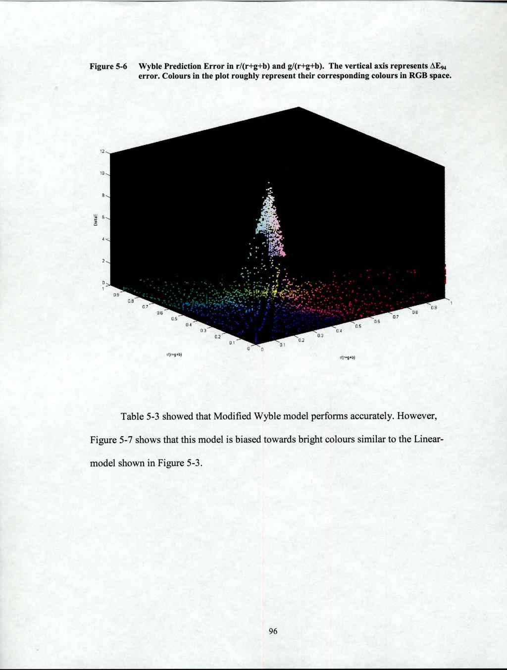
112

113 Figure 5-7 Wyble Modified Rediction Error in r/(r+g+b) and g/(rkg+b). The vertical asis represent AE94 error. Colours in the plot roughly represent their corresponding colours h RGB space. Figure 5-8 shows error of the Masking Model in chromaticity space. It is interesting to observe that this model is less biased towards bright colours and seems to have relatively similar performance for all the colours.

114 Figure 5-8 Masking Model Error in r/(r+g+b) and gl(r+g+b). The vertical axis represent AE94 error. Colours in the plot roughly represent their corresponding colours in RGB space. DeileE prediction using RGBCMYK method Comparing the backward error is more interesting. As shown in Table 5-4 The Masking Model outperforms Wyble in the backward direction. Backward error is calculated by predicting RGB values for a given XYZ input and the applying the forward model to predict the XYZ of the RGBbackward. The difference between the input and predicted XYZ is used to calculate AEg4 and the error is adjusted by subtracting data fiom forward model. Modified Wyble Modified is used to calculate XYZ output of RGBbhd for Wyble Model.

115 Table 5-4 Backward Error in AEY4 Wyble Masking Mean Dlp-Toshiba Max Std Mean Dlp-lnfocus Max Std Figure 5-9 and Figure represent error distribution of the two model for forward and backward prediction.

116 Figure 5-9 Distribution of Forward and backward error for Wyble Model. Left and right columns represent the forward and backward error distributions respectively. Top and bottom rows represent the dlp-toshiba and dlp-infocus displays.

117 Figure 5-10 Distribution of Forward and backward error for the Masking Model Left and right columns represent the forward and backward error distributions respectively. Top and bottom rows represent the dlp-toshiba and dlp-infocus displays. From the above results, we can conclude that both the Modified Wyble and Masking Models are accurate in predicting XYZ, while the Masking Model is the best choice for going backward Summary of DLP Calibration We compared possible spaces in which DLP calibration could be applied and we found that the RGBW and RGBCMYK spaces derived from RGB space can predict tristimulus values well. Wyble introduced a model that uses a 3x4 matrix to predict XYZ

118 values. A simple modification to his model can improve forward prediction accurracy. The Masking Model has similar error performance to the modified Wyble model in forward prediction (RGB to XYZ). However, we found that the Masking Model is not biased towards non-bright colours; whereas, the Wyble Model has really good performance for dark colours but its performance gets worse as the colours have a higher RGB value. Going backward, the Masking Model performs better than Wyble model in predicting RGB values. 5.4 DLP Projector Gamut In this section, we study the gamut of DLP projectors and consider which GMAs discussed earlier are the best choices for DLP displays. Figure 5-11 and Figure 5-12 represent the gamut shape of the two projector in XYZ space. These two figures show that DLP projectors clearly have a concave gamut. The white-filter effect can be assumed as the main reason for causing the concavity in DLP gamut. Interestingly, the projectors have a very similar looking gamut.

119 . I Figure 5-11 Gamut shape of dlp-infocus. Infocus DLP Gamut in xyz space 1 Figure 5-12 Gamut of dlp-toshiba -

120 Figure 5-13 Shows gamut of dlp-toshiba in CIELAB space, which similarly represents a concave shape gamut. Figure 5-13 dlp-toshiba gamut in CIELAB colour space. dlp-tosh~bs ~n L.seb'opece To understand why concavity occurs in DLP gamuts and we can consider the projectors Channel Interaction (CI). Figure 5-1 shows that blue and green channels have a different CI behaviour depending on whether the other two channels are set to maximum or not. This means that the tristimulus output of the ramps of blue and green are not

121 completely additive effect of the 3 primaries (red, green and blue lights), and there are some additional factors (in this case the white filter) that makes them behave differently. Since the red channel has a consistent CI, mostly increasing, independent of the other two channel settings, we can expect that the gamut boundary created by the ramps of red channel to have a convex shape. On the other hand, we should expect concavity on parts of the gamut with ramps of blue and green, since some artificial factor made their channel interaction to behave differently. This effect is shown in Figure 5-14, where the red and blue dots represent ramps of Red and Blue, respectively, while the other two channels are - set to maximum. Figure 5-14 Ramps of Red and Blue on the gamut when the other two channels are set to maximum.

122 This figure shows that on the part with ramps of red, the gamut is quite convex compared to the part with blue ramps. This is an interesting observation since it allows us to predict possible locations in the gamut that are likely to be concave. Extending this idea to the printer technology can be quite useful especially since studying printer gamuts with 7 or more inks is quite challenging. For printers, concavity can occur because of the ink-interaction and the inkseparation. Ink separation tells what ink combination to put down for a given RGB value. By studying the CI of RGB input values, we may be able to predict concavities that occur because of the ink-separation. Being able to remove these concavities can allow for expansion of the gamut and predicting the gamut boundary more accurately.

123 CHAPTER 6: LCD PROJECTOR VERSUS DLP PROJECTOR In this section, we compare some of the characteristics of LCD and DLP projectors. In particular, two of the main projectors characteristics are Temporal Stability and Spatial Non-Uniformity. In this study, two LCD and two DLP projectors were used. Table 6-1 shows the projector names used in this study. Table 6-1 Projector names used I 1 I Name Description PR1 PR2 Proxima LCD Desktop Projector 9250 Proxima LCD Ultralight LX dlp-toshiba Toshiba TDP-5 DLP Projector dlp-infocus Infocus DLP LP 1 Projector 6.1 Temporal Stability Temporal Stability indicates the amount of time it takes for the projector bulb to stabilize after it is turned on [42]. Full Red, Green and Blue were measured every 5 seconds for 45 minutes starting from the time that the projector was turned on. To improve the quality of the data, we made sure that before each test, projectors had been turned off for at least 5 hours for the bulbs to cool down. Figure 6-1 shows that Green and Blue channels have a big shift in their chromaticity as the LCD bulb warms up. On

124 the other hand, DLP projectors seem to have stable chromaticity fiom the very beginning, when they are first turned on. Figure 6-1 Temporal Stability for 2 LCD and 2 DLP projectors. In the first 3 columns, changes in R, G and B channels are shown. Horizontal Access represents d(x+y+z) and y/(x+y+z). Vertical access represents the data measurements. pr2 PR? PR2 Intensity dipinfocus Intensity apt- '+t@=f- - dlptmhiba Intensity