CMOS-MEA5000-System Manual

Transcription

1 CMOS-MEA5000-System Manual

2 Imprint Information in this document is subject to change without notice. No part of this document may be reproduced or transmitted without the express written permission of Multi Channel Systems MCS GmbH. While every precaution has been taken in the preparation of this document, the publisher and the author assume no responsibility for errors or omissions, or for damages resulting from the use of information contained in this document or from the use of programs and source code that may accompany it. In no event shall the publisher and the author be liable for any loss of profit or any other commercial damage caused or alleged to have been caused directly or indirectly by this document Multi Channel Systems MCS GmbH. All rights reserved. Printed: Multi Channel Systems MCS GmbH Aspenhaustraße Reutlingen Germany Phone Fax Microsoft and Windows are registered trademarks of Microsoft Corporation. Products that are referred to in this document may be either trademarks and/or registered trademarks of their respective holders and should be noted as such. The publisher and the author make no claim to these trademarks.

3 Table of Content Table of Content... 3 Important Safety Advice... 5 Guarantee and Liability... 6 Operator's Obligations... 6 Introduction... 7 Welcome to the CMOS-MEA5000-System... 7 Hardware... 8 Headstage... 8 CMOS MEA Chip... 9 MCS-IFB 3.0 Multiboot Interface Board Hardware Setup Installation of the Software System Requirements Testing the CMOS-MEA5000-System Functional Tests of the CMOS-MEA5000-System with the Test Model Probe General Software Features CMOS-MEA-Control Introduction Main Window Menu Bar Control Section Data Display Activity Sensor Array Tool Spike Tool Stimulation Analog Channels Digital Port Events Detailed View: Region of Interest Single Sensor View Operating CMOS-MEA-Control Recording Stimulation CMOS-MEA-Tools Main Window Menu Bar Tool Bar Analysis Control Window Data Display and Settings Window Filter Raw Data Explorer Spike Explorer Window STA Explorer Window Spike Sorter Tool User Interface Processing View Chip Overview ROIs in Progress Log Remote Sorting Clients

4 Results View Toolbar Units List Filters and Sorting Chip Overview Unit Comparison Unit Details Spike Sorter Settings ROIs Computing Sorting Peak Detection Post-Processing Presets Spike Sorting Client Spike Sorter Client on Linux File Format Tutorials Running a Spike Sorting Analysis Identifying Units from the UI Adjusting the Spike Sorter Sensitivity Increasing the Sensitivity to find more Units Avoiding Noise Units Memory Issues Distributed Spike Sorting Converting Raw Data to Units Spike Sorting Algorithm Basic Principles Independent Component Analysis (ICA) Main Processing Steps Extract Regions of Interest Extract Units from a Region of Interest Remove Redundant Units Unit Quality Measures SNR Skewness Kurtosis AmplitudeSD RSTD Separability IsoIBg and IsoINN References Support and Troubleshooting Troubleshooting Technical Support Technical Specifications CMOS-MEA Chip Test-CMOS-MEA Contact Information Index

5 Important Safety Advice Warning: Make sure to read the following advice prior to installation or use of the device and the software. If you do not fulfil all requirements stated below, this may lead to malfunctions or breakage of connected hardware, or even fatal injuries. Warning: Always obey the rules of local regulations and laws. Only qualified personnel should be allowed to perform laboratory work. Work according to good laboratory practice to obtain best results and to minimize risks. The product has been built to the state of the art and in accordance with recognized safety engineering rules. The device may only be used for its intended purpose; be used when in a perfect condition. Improper use could lead to serious, even fatal injuries to the user or third parties and damage to the device itself or other material damage. Warning: The device and the software are not intended for medical uses and must not be used on humans. Malfunctions which could impair safety should be rectified immediately. High Voltage Electrical cords must be properly laid and installed. The length and quality of the cords must be in accordance with local provisions. Only qualified technicians may work on the electrical system. It is essential that the accident prevention regulations and those of the employers' liability associations are observed. Each time before starting up, make sure that the power supply agrees with the specifications of the product. Check the power cord for damage each time the site is changed. Damaged power cords should be replaced immediately and may never be reused. Check the leads for damage. Damaged leads should be replaced immediately and may never be reused. Do not try to insert anything sharp or metallic into the vents or the case. Liquids may cause short circuits or other damage. Always keep the device and the power cords dry. Do not handle it with wet hands. Requirements for the Installation Make sure that the device is not exposed to direct sunlight. Do not place anything on top of the device, and do not place it on top of another heat producing device, so that the air can circulate freely.

6 Guarantee and Liability The general conditions of sale and delivery of Multi Channel Systems MCS GmbH always apply. They can be found online at and Conditions.pdf Multi Channel Systems MCS GmbH makes no guarantee as to the accuracy of any and all tests and data generated by the use of the device or the software. It is up to the user to use good laboratory practice to establish the validity of his / her findings. Guarantee and liability claims in the event of injury or material damage are excluded when they are the result of one of the following: Improper use of the device. Improper installation, commissioning, operation or maintenance of the device. Operating the device when the safety and protective devices are defective and/or inoperable. Non-observance of the instructions in the manual with regard to transport, storage, installation, commissioning, operation or maintenance of the device. Unauthorized structural alterations to the device. Unauthorized modifications to the system settings. Inadequate monitoring of device components subject to wear. Improperly executed and unauthorized repairs. Unauthorized opening of the device or its components. Catastrophic events due to the effect of foreign bodies or acts of God. Operator's Obligations The operator is obliged to allow only persons to work on the device, who are familiar with the safety at work and accident prevention regulations and have been instructed how to use the device; are professionally qualified or have specialist knowledge and training and have received instruction in the use of the device; have read and understood the chapter on safety and the warning instructions in this manual and confirmed this with their signature. It must be monitored at regular intervals that the operating personnel are working safely. Personnel still undergoing training may only work on the device under the supervision of an experienced person

7 Introduction Welcome to the CMOS-MEA5000-System Multi Channel Systems is proud to present the CMOS-MEA5000-System. Based on the complementary metaloxide semiconductor technology, it opens up new possibilities in electrophysiological research. With more than 4000 recording sites, each of them sampled at up to 25 khz, the chip allows extracellular recordings at a very high spatio-temporal resolution. By including amplification on the chip itself, noise is minimized and a high signal quality is guaranteed. Stimulation is provided via 1024 stimulation sites included in the chip and the stimulus generator in the headstage. The CMOS-MEA5000-System consists of three components, which are all designed to be efficient and powerful, while maintaining a small footprint. CMOS-Chip The chip is based on complementary metal oxide semiconductor (CMOS) technology, facilitating fast, high resolution imaging of electrical activity. The chip is equipped with a culture or slice chamber to house your sample, while allowing the use of a microscope. Headstage The core of the system is the headstage. It samples the data coming from the chip at 25 khz per channel. Besides A/D conversion and amplification, the headstage also houses a three-channel stimulator. You can freely design the stimulation patterns via software and select each of the 1024 stimulation sites. Interface Board The interface board offers the USB 3.0 interface to transfer the recorded data to a computer. Moreover, it has analog and digital in- and outputs for synchronization with other instruments. Computer with Software The software CMOS-MEA-Control and CMOS-MEA-Tools are programmed specifically for the CMOS- MEA5000-System. It facilitates a real-time activity overview on the complete chip with the ability to zoom in and various tools to analyze the data

8 Hardware Headstage There are three hardware components for the CMOS-MEA5000-System available, the headstage, the interface board and the data acquisition computer. If necessary you can use a temperature controller additionally. For setting up and connecting the CMOS-MEA5000-System, please read the next chapter "Hardware Setup" on page 15. The headstage samples data coming from the 4225 sensors on the chip at 25 khz per channel. Besides A/D conversion and amplification, the headstage also houses a three-channel stimulator. You can freely design three stimulation patterns via software and select each of the 1024 stimulation sites. Insert the test model probe or the CMOS-MEA-Chip in correct orientation into the provided area in the headstage. The round edge of the probes have to be in the front on the left, when looking directly to the open headstage. Data transfer is provided via SATAp cable from the headstage and to the MCS Interface Board. The USB 3.0 cable connection arranges fast data transfer from the interface board to the data acquisition computer. Connect a temperature controller TC to the headstage, if necessary

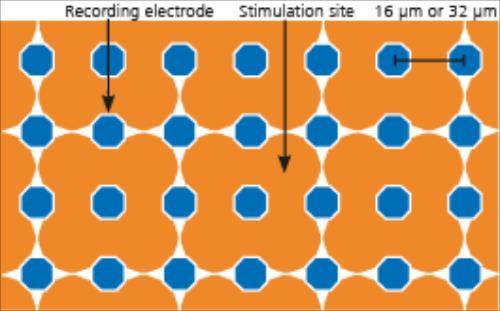
9 CMOS MEA Chip The chip is based on complementary metal oxide semiconductor (CMOS) technology, facilitating fast, highresolution imaging of electrical activity. The chip is equipped with a culture chamber to house your sample, while allowing the use of a microscope. The CMOS MEA array is an active device, in contrast to the passive MEAs. It needs to be powered up and down properly, or it will be damaged. Warning: Before opening the CMOS-MEA headstage for removing the CMOS MEA chip, it is necessary to power the chip down, otherwise the chip will be destroyed! CMOS sensor arrays are light sensitive. During recording the sensors need constant light conditions. This is easy to obtain by covering the CMOS array with an inverted petri dish, for example, which is wrapped in aluminum foil. The CMOS MEA chip has a 65x65 layout and is available with 16 μm or 32 μm interelectrode distance (center to center). The electrode diameter is always 8 μm. Between the recording electrodes, there is a grid of 32 x 32 bigger stimulation sites. Summarizing, you can record from 4225 electrodes and stimulate your sample at 1024 sites. The chip is coated with a planar oxide, similar to glass, enhancing the biocompatibility and biostability. Please see the electron micrograph of the CMOS MEA chip surface (NMI Reutlingen, Germany) above and the schema of the chip below

10 The 16 μm interelectrode distance chip offers the highest resolution. With the high number of electrodes, you can record from a large surface (1 16 μm distance, 4 32 μm distance). Thereby, you can see the signals from every single cell and even the signal propagation along an axon, while still getting an overview on your complete sample. Your data is sampled at up to 25 khz per channel. Thus, no signal is lost - even axonal spikes are displayed and recorded thoroughly. Together with the A/D conversion at 14 bit, the system ensures accurate and precise data. At the moment three types of culture chambers are available for CMOS-MEAs: One for cell cultures and two for acute slices. CC Culture chamber for cell cultures with lid. SCB Slice chamber basic. Additionally a CMOS-MEA chip with a SCA Slice chamber advanced is available

11 MCS-IFB 3.0 Multiboot Interface Board The interface board (IFB) offers the USB 3.0 interface to transfer the recorded data to a computer. Moreover, it has analog and digital in- and outputs for synchronization with other instruments. Connect the headstage via esatap cable to the interface board. Connect the interface board via USB 3.0 to the data acquisition computer. Connect the interface board to the power outlet. Ground the interface board if necessary. Please use the ground socket on the rear panel of the IFB. Front Panel Two Status LEDs The status LEDs indicate the link status of the CMOS-MEA headstage. They light up when the headstage is connected to the interface board via esatap cable. LED 1 lights up, when connecting the headstage to connector 1 on the side panel of the IFB, which is recommended, LED 2 in on when using connector 2. Important: Please use connector labelled "1" on the side panel of the IFB and USB plug in labelled "A" on the rear panel of the IFB, otherwise the headstage will not work. Auxiliary Channels Two reserve auxiliary channels are available for future use. They have no function at the moment. Digital IN / OUT A Digital IN / OUT for 16 digital in- and output bits is available (68-pin MCS standard connector) on the rear panel of the interface board. The Digital OUT delivers TTL pulses with 3.3 V. On the front panel four digital IN and four digital OUT connectors bits are also accessible via Lemo connector DIG IN bit 0 to bit 3 and DIG OUT bit 0 to bit 3. If access to more bits of the DIG IN / OUT channel is required, it is necessary to connect a Di/o board with a 68-pin standard cable. This Di/o board is available as optional accessory

12 Power LED The power LED near to the MCS logo on the front panel of the interface board should light up when the CMOS-MEA5000-System is "ON", and the device is connected to the power line. If not, please check the power source and cabling. Rear Panel Toggle Switch On / Off Toggle switch for turning the device on and off. The CMOS-MEA5000-System is switched to status "ON" when the toggle switch is switched to the left. The device is switched "OFF" when the toggle switch is switched to the right. If the system is "ON", and the device is connected to the power line, the Power LED on the front panel of the interface board should light up. If not, please check the power source and cabling. Power IN Connect the power supply unit here. This power supply powers both, the headstage and the interface board of the CMOS-MEA5000-System. The device needs 12 V and 2.5 A / 30 W. Ground If an additional ground connection is needed, you can connect this plug with an external ground using a standard common jack (4 mm). Digital IN / OUT A Digital IN / OUT for 16 digital in- and output bits is available (68-pin MCS standard connector). Please read chapter "Pin Layout" (Digital IN / OUT Connector) in the Appendix for more information about the pin layout of the connector. The Digital IN / OUT connection accepts or generates standard TTL signals. TTL stands for Transistor-Transistor Logic. A TTL pulse is defined as a digital signal for communication between two devices. A voltage between 0 V and 0.8 V is considered as a logical state of 0 (LOW), and a voltage between 2 V and 5 V means 1 (HIGH). The Digital OUT delivers TTL pulses with 3.3 V. The Digital OUT allows generating a digital signal with up to 16 bits and read it out, for example, by using a Digital IN / OUT extension Di/o from Multi Channel Systems MCS GmbH. You can utilize this digital signal to control and synchronize other devices with the CMOS-MEA5000-System. Bit 0 to 3 of the Digital OUT are separated and available as Lemo connector DIG OUT 0 to 3 on the front panel of the interface board. So if you need only one, two, three or four bits of the digital signal, you don t need the additional Di/o. Please read chapter "Pin Layout" (Digital IN / OUT Connector) in the Appendix for more information. The Digital IN can be used to record additional information from external devices as a 16 bit encoded number. The Digital IN is most often used to trigger recordings with a TTL signal. The 16 bit digital input channels is a stream of 16 bit values. The state of each bit (0 to 15) can be controlled separately. Standard TTL signals are accepted as input signals on the digital inputs

13 Warning: A voltage that is higher than +5 Volts or lower than 0 Volts, that is, a negative voltage, applied to the digital input would destroy the electronics. Make sure that you apply only TTL pulses (0 to 5 V) to the digital inputs. Analog Channels Eight Analog IN channels are available via 10 pin connector. Please read chapter "Pin Layout" (Analog IN Connector) in the Appendix for more information. The additional analog inputs are intended for recording additional information from external devices, for example, for recording patch clamp in parallel to the MEA recording, for monitoring the temperature, or for fluidic control. Two of these channels (No 1 and 2) are available via Lemo connectors on the rear panel of the interface board. You could also use the analog inputs for triggering, but please note that the digital inputs DIG IN 0 to 3 are intended for accepting TTL pulses. Signals on the analog channels are digitized and amplified with a gain factor of 2. Analog Channels 1 and 2 Two of the eight analog channels described above (analog channel 1 and 2) are directly accessible via two Lemo connectors. DSP JTAG Connector The 20-pin JTAG connector is used to program the digital signal processor DSP for real-time feature. This feature is not in use in CMOS-MEA5000-Systems. USB 3.0 Connector The USB connector is used to transfer the amplified and digitized data from all data channels and the additional digital and analog channels to any connected data acquisition computer via USB 3.0 high speed cable. The USB cable has to be connected to the USB port labelled with "A" on the rear panel of the interface board. Important: It is recommended to connect the USB 3.0 high speed cable direct to the USB 3.0 port of the computer. Do not use an USB hub! Audio OUT The "Audio OUT" function is not available for the CMOS-MEA5000-System. Side Panel Sockets for connecting the CMOS-MEA5000 headstage via esatap cable to the interface board MCS-IFB 3.0 Mulitboot. Please use the connector labelled with "1"

14 Data Acquisition Computer The software CMOS-MEA-Control was programmed specially for the CMOS-MEA5000-System. It facilitates a real-time activity overview on the complete chip with the ability to zoom in and various tools to analyze the data. Please read chapter "CMOS-MEA-Control" for information about the software. The data acquisition computer is provided by Multi Channel Systems MCS GmbH. The operation system Windows 8.1 is necessary. Due to the huge amount of recorded data, a computer with low performance may lead to performance problems; therefore, Multi Channel Systems provides an up-to-date computer with USB 3.0 connection and Intel chip set. Use a SSP hard drive for recording and a second hard drive for backup. At full frame sampling with maximum sampling rate the currently used 1TB SSD drive will hold about one hour of continuous recording only!

15 Hardware Setup Please follow the instructions: 1. Connect the CMOS-MEA5000 amplifier via esatap cable to the MCS IFB interface board. Please use the plug in labelled with 1 on the side of the interface board. 2. Connect the MCS IFB via power unit to the power outlet. 3. Connect the MCS IFB via USB 3.0 to the computer. Use the USB plug in labelled with A on the backside of the interface board. 4. Connect the MCS IFB via USB 3.0 cable to the backside of the computer. It is mandatory to use the designated USB 3.0 port, please see the picture below! Important: It is necessary to connect the interface board of the CMOS-MEA5000-System MCS-IFB 3.0 Multiboot to an Intel USB 3.0 port. Otherwise you risk data loss

16 Please consider the error message when starting the CMOS-MEA-Control software for the first time. Important: Make sure that all paths for recording files go to the SSD drive otherwise no recording is possible! 5. Connect the temperature controller TC via USB 2.0 high speed cable to one of the USB 2.0 ports and via power unit to the power outlet. 6. Connect the heating element of the CMOS headstage via provided cable to the temperature controller

17 Installation of the Software System Requirements If you have purchased the CMOS-MEA5000-System with PC everything is preinstalled and tested. If you purchase a system without a PC please make sure that the computer meets our specifications relating processor, memory, hard disk, etc. Please contact Multi Channel Systems MCS GmbH or your local retailer. Software: One of the following Microsoft Windows operating systems is required: Windows 10 or 8.1, 64 Bit (English and German versions supported) with the NT file system. Other language versions may lead to software errors. Due to the amount of recorded data, a computer with low performance may lead to performance problems; therefore, Multi Channel Systems MCS GmbH recommends an up-to-date computer. Please contact MCS or your local retailer for more information on recommended computer hardware specification. Important: Because of the huge amount of acquired data (up to 220 MByte per second), make sure that all paths for recording files go to the SSD drive, otherwise no recording is possible! Please note that there are sometimes hardware incompatibilities of the data acquisition system and computer components; or that an inappropriate computer power supply may lead to artefact signals. Recommended Operating System Settings The following automatic services of the Windows operating system interfere with the data storage on the hard disk and can lead to severe performance limits in CMOS-MEA-Control. These routines were designed for use on office computers, but are not very useful for a data acquisition computer. Deselect "Windows Indexing Service" for data SSD and HD disks, the system hard drive is not included. Switch off the sleep mode for displays and HD disks. Power Options: Power scheme: High performance. Never turn on system standby. Turn off "Optimize hard disk when idle", the automatic disk fragmentation. Turn off the Screen Saver and do not use a virus scanner during experiment. It is also not recommended to run any applications in the background when using CMOS-MEA-Control. Remove all applications from the "Autostart" folder. Important: Please make sure to have full control over your computer as an administrator. Otherwise, it is possible that the installed software does not work properly. Doubleclick the CMOS-MEA-Control.exe on the installation volume. The installation assistant will show up and guide you through the installation procedure. Follow the instructions of the installation assistant. Note: During installation all drivers are installed and if necessary the firmware of the CMOS-MEA5000 hardware is updated. Please do not interrupt the firmware update

18 Testing the CMOS-MEA5000-System Functional Tests of the CMOS-MEA5000-System with the Test Model Probe Please read also the datasheet "Test CMOS-MEA" in the Appendix. Insert the "Test Model Probe" in correct orientation and close the headstage. The round edge of the Test-CMOS-MEA or the CMOS-MEA chip has to be in the front on the left side when looking directly to the open amplifier. The provided test model probe simulates a CMOS-MEA chip with a resistor of 100 k and a 10 p capacitor between ground and each row of the 65 x 65 electrodes in the grid. It can be used for testing the noise level of a CMOS-MEA5000-System, for a test of calibration and for testing the internal stimulators. CMOS-MEA test model probes and CMOS-MEA chips are active devices and must be switched on and shot down properly, otherwise they might suffer damage. Please click the MEA array icon in the "Data Source" window. CMOS chips must be calibrated before each use. The calibration runs automatically and usually takes two to three minutes. Please do not interrupt the process, until the final message "Finished automatic system calibration" appears. The Test CMOS-MEA simulates the calibration of the chip. The ODD cable supports the odd-numbered channels and the EVEN cable supports the even-numbered channels. For the intention to check the noise level of a CMOS-MEA5000-System without external signals, please connect the cable soldered to the ODD connector to the input connector of the even-numbered channels and the cable soldered to the EVEN connector to the BATH input. Connected in this way, the signal input supports all 65 rows of the 65 x 65 layout of the CMOS-MEA chip at a time and simulates also the calibration of the bath. Disconnect the "ODD" connector to see the "EVEN" numbered electrodes only and vice versa to see the "ODD" numbered electrodes only

19 Test of the internal Stimulators The Test-CMOS-MEA probe is equipped with three additional connectors to test the internal stimulation, STG1, STG2 and STG3. The stimuli are color coded in the CMOS-MEA-Control software: Stimulus 1 is indicated in green color, Stimulus 2 is indicated in blue and Stimulus 3 in red color. For testing a stimulator, please connect the cable of the "ODD" connector to the "EVEN" connector and the open cable to one of the "STG" plug ins. Define a respective stimulus pattern in the "Stimulation" window, for example a ramp with 100 ms on stimulator 1 (green), as shown on the screenshot above

20 CMOS-MEA Chip Please fill the CMOS-MEA chip with PBS and add an external reference electrode. CMOS sensors are light sensitive. To record a stable baseline the CMOS-MEA array must maintain under stable light conditions, which can easily be provided by covering the CMOS-MEA with aluminum foil. Otherwise the signal will drift out of range by the effect of light

21 General Software Features The chapter "General Software Features" describes some of the CMOS-MEA-Control and CMOS-MEA-Tools software features on base of examples. Numeric Up-Down Box Adjust a value in the numeric up-down box either by clicking on the arrow buttons or by clicking into the window and moving the mouse wheel. Turn the wheel forward and the level increases, turn the wheel backward and the value decreases in fast steps. Use the arrow buttons for fine tuning the adjustment. The third possibility is a replacement of the number in the window by overwriting it, if the value is predefined, for example. Zoom In and Zoom Out Zoom Buttons Click the "Adjust to signal Min/Max" button. The scaling of the y-axis is set to the minimum and maximum of all visible samples in the channel. Click the "Zoom" buttons. Zooming in cuts the scaling of the respective axis in a half and zooming out doubles the scaling. Zoom by Mouse-click Additionally to the zoom buttons you can freely zoom into a region of interest by moving the mouse inside a display from the left to the right while pressing the left mouse button. Move the mouse from the right to the left for zooming out

22 Display Floating Design your own display with the floating feature. Decouple a dialog display of your choice and place it wherever you want. Dock the window again by clicking with the right mouse button on top of the window. Hide a window with the "Auto-Hide" option. Creating Regions of Interest ROIs Selecting ROIs manually by drawing rectangles is identical even in the "Activity" or "Sensor ArrayTool" window. Please keep the left mouse button pressed to draw a rectangle in the "Activity" window to create a region of interest. A dashed line in blue indicates the borders of the ROI. The color of the rectangle turns to black and the ID of the ROI appears in the upper right edge. Or create a ROI by clicking on one of the activity maxima. Modify a region of interest be clicking on the borders until a double arrow appears to move the border. Delete a ROI by clicking on the ROI again. The sensor channels included in a region of interest are immediately shown in the "ROI" window beside

23 CMOS-MEA-Control Introduction The software for controlling the CMOS-MEA5000-System includes two parts, CMOS-MEA-Control for online recording, CMOS-MEA-Tools for offline analysis. The CMOS-MEA-Control software is explicit designed for online data recording with the CMOS-MEA5000- System. It facilitates a real-time activity overview on the complete chip with the ability to zoom into the raw data and various tools to visualize the activity. The CMOS-MEA-Control software controls the CMOS-MEA5000-System, the experimental procedure, the data selection for recording to hard disk and similar functions like the control of stimulation, the online spike detection, the saving of spikes with or without raw data to save disk space or the selection of regions of interest selection for data reduction and many additional functions. Main Window

24 The default window of the main menu is divided in three parallel sections which are framed by the menu bar above: 1. Left: Control section to control the CMOS-MEA5000-System hardware, the data acquisition, the experimental procedure, the recording of data, the streaming of detected spikes and a section to monitor the system load. 2. Middle: Tools section with tools to set sensor array properties, to monitor the acquired data online, to detect spikes, to stimulate and to extract events from a digital input signal. 3. Right: Data view section with detailed views of the raw data or of detected spikes. You can zoom into the data in a region of interest above and in a detailed single view of one recording electrode below. Menu Bar File Menu to open and to save templates and to "Exit" the program. Settings Menu to activate the "Tools", "Activity Tool" and "Spike Tool". Switch the tools on via check box in order to perform their respective tasks or off to reduce the system load. When the "Activity Tool" is switched off no raw data will be displayed, but of course processed and stored. When the "Spike Tool" is switched off no spike detection is performed and no spikes are stored. Note, that the spike detection on so many sensors is an expensive task and needs an appropriate computer

25 Menu to "Set Default Folder", to "Save Default Folders" and to "Clear Defaults". Define the paths for the "Default Folders" for "Raw Data", "Template" and "Stimulation Files" in the "Application Settings" dialog. Important: Make sure that all paths go to the SSD drive otherwise no recording is possible! Lab Book Please use entries in the three tabs of the lab book for later analysis of the experiment. Click the button "Set Default" for keeping the information as template. All notes will be saved in the raw data file

26 Setup Click "Device" to change the connected device. If hardware is available, choose the "MCS Device". If no hardware is available, please use the "Simulator" or load a "Data File" to test the software without hardware attached. When replaying a data file you have the advantage to see "real" data meanwhile the data of the "Simulator" are virtual. To select a data file from a folder, please choose "Data File" in the "Setup" menu. The "Data Source" window displays "Simulation" beside the CMOS-MEA5000-System button. Then click on the CMOS MEA chip button to select the file you want to replay from the browser dialog. Click "CMOS System" to open the "Setup CMOS System" dialog

27 "Setup CMOS System" dialog provides the manual control for the offset and calibration settings for the CMOS chip. There is an automatic routine for the chip start up and calibration, the manual settings are usually not needed. Please read chapter "Operating the CMOS-MEA-Control Software" for detailed information. Open the "Device Filter" dialog to change filter settings. Adjust the settings of the "High Pass" and "Low Pass" filter on hardware level during the software is running, but not recording. Choose "Bessel" or "Butterworth" filter "Family" in 1 or 2 "Order" from the drop-down menus. Switching "Off" the "Cutoff Frequency" of the high pass filter enables DC signals. If filter settings should be saved for later experiments, please click the "Set Permanent" button. Help When starting the CMOS-MEA-Control software this pop-up "Software Update Available" appears, when a new version of the software is available. Click on the note to open the "Check for Updates" dialog to have direct and fast access to the MCS web site

28 If the software is not up to date, click the button "Visit Web site" and download the newest software version. The "Help" menu is for opening the online help "CMOS-MEA-Control Help" and to "Download Update", if necessary. Click the "About" option for software and firmware information. Please see technical specifications of the device and the version number of the CMOS-MEA-Control software

29 Control Section The "Control Section" includes three sections, the "Data Source", the "Recorder" and the "Load" control. Data Source The "Data Source" window allows controlling the data source and the CMOS chip. The chip is an active device and has to be powered before you are able to start an experiment with the "Start" button. Click the "Settings" icon for the "Set Device" dialog. When using a CMOS-MEA5000-System for the first time, please define which CMOS MEA "Device" is currently in use and define the "Sample Rate" from the drop-down menus. Selecting "Analog Channels" and the digital "Digital Channel" enables the selected channels. Decide in the "Recorder" window whether you want to record from these channels or not, please see the next screenshot

30 Recorder Control the "Recorder" parameter settings in this window. Start and stop the recorder and see the types of data available. Press the "Settings" icon to change recorder settings. Please read chapter "Operating CMOS-MEA-Control" for detailed information about programming the recorder. Start and stop the recording manually with the "On/Off" icon. When the recorder is running, the recording time and the path where to store the data file is displayed. Define this data path in the "Recorder Settings" dialog. Define additionally the "File Name" and the "Prefix" and "Suffix". Start and stop the recorder in three different modes: In "Manual" mode, via "Timer" or in dependency of an "Event". Please read chapter "Operating CMOS-MEA-Control" for detailed information

31 Spike Server The "Spike Server" allows to stream detected spikes and events to other applications on the same computer or to another computer in the network. The client receives the data and can process it to the needs of the customer. We provide source code for such a client in C#, Matlab and Pythen. Load Monitor the current state of the capacity of the data acquisition computer via "Load" window. See the CPU load in "CPU Usage", and most important the available "Disk Space" on the drive used for recording. Note that the CMOS-MEA5000-System generates up to 220 MB per second when recording with maximum sample rate! The "Data Source" and "Recorder", the "Activity Tool", the "Spike Tool" and the "Spike Server" window allow to see which components of the software are generating which amount of processor load at the moment. Each tool has its own queue of data packages to process. If the load of the processor is high tools may not be able to process its data and the data queue of the tool grows. This state of the queue is shown for each tool separately

32 Sensor Current See the "Sensor Current" of the CMOS chip. The sensor current is measured as the sum of all current over all 4225 sensors. The total current should not be larger than about 300 ma, otherwise the chip get damaged. Log The "Log" file window displays the ongoing experimental proceedings online. In the "Log" file all software operations during an experiment are documented. The "Log" can be saved and exported as "*.xml" file by pressing the disc icon

33 Data Display Activity Due to the high number of channels, it s impossible to show raw data of 4225 channels simultaneously. Therefore, activity is visualized in time bins in a false color code. This allows the user to identify active areas and to focus on them in regions of interest. Display the "Activity" data in three modes: "Mean Amplitude", "Max Amplitude" and "Spike Count". See the complete CMOS MEA electrode array in the "Activity" window. The "Activity" plot shows all 65 x 65 sensors of the CMOS chip as one pixel each. Select as much "Regions of Interest ROIs" as needed to display the most exciting regions of the CMOS array only. In the screenshots below regions of interest are displayed

34 Creating Regions of Interest ROIs Please keep the left mouse button pressed to draw a rectangle in the "Activity" window to create a region of interest. A dashed line in blue indicates the borders of the ROI. The color of the rectangle turns to black and the number of the ROI appears in the upper right edge. Or create a ROI by clicking on one of the activity maxima. Modify a region of interest be clicking on the borders until a double arrow appears to move the border. Delete a ROI by clicking on the ROI again. Regions of interest are displayed in separate tabbed pages. To switch from one ROI to another, please use the tabs under the "Single View" of the "ROI" window. Important: It is not allowed to overlap regions of interest! The sensor channels included in a region of interest are immediately shown in the "ROI" data window beside. The toolbar of the "Activity" is divided into two parts: One part above and one part below the "Activity" display

35 Upper Toolbar of the "Activity" Window Click the "Parameter Selection Icon" icon to decide which parameter mode of the sensor activity should be displayed: The maximal "MaxAmplitude" or the "MeanAmplitude or the "SpikeCount". In dependency of your choice, the toolbar beside changes. The selected parameter will be shown in the activity window as false color plot in time bins. Define the color of the map in the "Sensor Array View Settings" dialog. For the "SpikeCount" parameter, spikes are detected individually for each channel by a threshold crossing. The threshold is calculated as standard deviation of the noise for that channel, as a user defined factor. The factor can be changed with the up-down box next to the parameter selection icon. The calculation of the standard deviation can be updated at any given time with the icon "Update the Std. Dev. Measure". Open the "Activity Tool Settings" dialog by clicking the icon. The basic parameters, like update of the time bins and the detection dead time can be changed in the "Activity Tool Settings" dialog. The "Update" parameter defines the size of the time bins and the refresh rate of the display. Accumulate and Detection Dead Time are important if the spike count is displayed. Spike count will be accumulated for the selected time, events crossing the detection threshold within the selected "Detection Dead Time" after a previous event will be ignored. This means that when looking at spike count, the display will begin to show data with a few seconds delay after starting the data acquisition, depending on the Accumulate setting

36 Lower Toolbar of the "Activity" Window If the mouse pointer is positioned on the map, the coordinates of the area the mouse is pointing at is shown at the left side of the toolbar below the plot window. Define the color of the "Activity Map" by clicking the second setting icon in the toolbar below. The "Sensor Array View Settings" dialog appears. Enable the check box "Invert" to invert the colors of the activity map. By default, one region of interest (ROI) is defined on the "Activity" display. The raw data of all sensors within the ROI is displayed in detail. The size and position of the ROI can be changed by dragging with the mouse. It is possible to define more than one region of interest. Click the buttons for adding or removing additional ROIs. Please draw a rectangle with the mouse over the respective sensor array to define the area of a ROI. If more than one region of interest is available, they are independently displayed in tabbed pages. Please read also chapter "Creating Regions of Interest ROIs" above. Optionally it is possible to define the area of a ROI with the "Set ROI Cursor" dialog. Define the "Position", "Size", and "Color" of the ROI cursor. Show or hide the cross hairs via "Show Cross Hairs" check box below and "Enable" the cursor via the check box above

37 Define the value of the color map in microvolt with the up-down box "Range". The maximum value should be close to the maximum amplitude or spike frequency of the expected signals. The color depicts the selected parameter in the "Activity" display. As seen in the image below, activity is shown as colored spots. Sensor Array Tool The "Sensor Array Tool" integrates three functions which are related to the control of the CMOS-MEA chip

38 First of all you can manually recalibrate your sensors, if necessary. Secondly, regions of sensors can be selected manually or automatically to focus only on interesting regions. Thirdly, when necessary the operating point of the sensors can be resetted by setting the appointed gate voltage once or in repeated mode anew. At the end of the system calibration run the conversion factors of all sensors which are displayed in order to evaluate the quality of the sensor chip. Please select one of the three modes from the drop down menu: "Calibration", "Sensor Selection" and "Sensor Reset". Calibration As mentioned above the condition of the sensor chip can be estimated by the conversion factors obtained during the system calibration. Each sensor's calibration value is represented by a color coded dot. The exact values depend on the sensor chip. The pattern of this values should be a kind of random noise pattern. Any structures within this random noise pattern may indicate a problem. For example, a white area may point to a group of defective sensors. Or a straight horizontal line across the whole chip indicates a bad contact to the sensor chip. Please stop the experiment and clean the contact pins of the headstage. White pixel point to a defective single sensor, where calibration was not possible. Try to repeat the process by clicking the "Calibrate" icon for the calibration of the CMOS sensors. This is the same command as in the "CMOS-MEA Diagnose" dialog. For calibration a sine signal with 70 Hz and 3 mv is set against a sine signal from the internal stimulator

39 Sensor Selection The "Sensor Selection" module allows the user to select regions of interests manually or automatically. It is useful to reduce the amount of data transferred to the computer and to hard disk when the activity is restricted to one or several locations of the sensor array. Fetch the activity distribution obtained by the "Activity" or "Spike Tool" and use it to define the regions of interest

40 Upper Toolbar of the "Sensor Array Tool" Window Please download your selection of regions of interest with the "Download the Selected Sensors to Data Acquisition" button to the computer. Use the "Fetch Spike Count from Spike Tool" button to import data from the "Spike Tool" and click the "Fetch Activity from Activity Tool" button to import data from the "Activity" tool. Lower Toolbar of the "Sensor Array Tool" Window Select the complete array with the "Select complete Sensor Array" button. Use the "Automatic Sensor Selection" button if you are not going to select the regions of interest manually. The automatic tool selects areas around activity peaks. Please define the dimension of the region of interest from the drop-down box, "Size 3 x 3" sensors or "Size 5 x 5" sensors. Deselect all regions of interest with the "Remove selected Sensors" button. Additionally to the automatic selection of ROIs you are able to add ROIs or to modify or to remove sensor arrays manually. Please read in chapter General Software Features" on page 21 paragraph "Creating Regions of Interest ROIs". Sensor Reset For very long recordings or for experimental conditions which causes strong potential drifts of the sensors it may be necessary to reset the sensors operating point. The reset of the sensors can be controlled manually or automatically at user defined intervals. The timing of the reset is acquired and saved as channel data and also as events together with the sensor data. This information can be used to exclude the reset phases from analysis

41 To reset the sensors operating points select the "Sensor Reset" module from the "Sensor Array Tool" toolbar. Press the start button to reset the sensors. The duration of the reset can be set with a numerical control. Check the "Repeat" control to automatically repeat the sensor reset with a given interval. The "Sensor Reset" tool raises the floating signals back to the operation point. This short period is visible in the raw data as a potential step. The exact time of the reset is recorded together with the raw data as channel data or as events. Example: "Sensor Reset" without suppression The example above on the left shows a sensor reset with an interval of 1 ms and no suppression. A filter of 10 Hz is applied. The example above on the right shows a sensor reset with an interval of 1 ms and no suppression without filter

42 Example: "Sensor Reset" with suppression The example above on the left shows a sensor reset with an interval of 1 ms, with 10 Hz filter and with suppression. The example above on the right shows a sensor reset with an interval of 1 ms, without filter and with suppression. The effect of the suppression and of the 10 Hz high pass filter is obviously to see in comparison of the four screenshots above

43 Spike Tool The "Spike Tool" is used for the online determination of spikes parameters

44 Spike Tool Toolbar Define the "Threshold" for the spike detection from the drop-down box: "Positive", "Negative" or "Absolute". Select the standard deviation "StdDev" from the numeric up-down box. Use the "Update StdDev Measure" feature, if necessary. Click the "Open Settings Dialog" button to open the "Spike Explorer Settings" dialog. The dialog has two tabbed pages

45 Spike Detection The noise is used as a base to calculate the threshold of the spikes which should be detected. "Noise Measure" parameter: Select whether you want to set the "Standard Deviation" or the "Median/Absolute Deviation" for noise measuring. "Timing": Three parameters are available to define the timespan in which the noise should be measured for using it as a base for the threshold. The "Continuous" measuring is opposed to the interval measuring. Use a "Single Interval" or "Repeat Interval". Continuous measuring of the noise as base for the spike threshold is necessary, if the raw data are drifting. This way, the threshold for the spikes will be adapted. To repeat the noise measure in intervals is also reasonable for ongoing experiments. Please define the number of "Repeat(s)" and the "Duration" of the interval in milliseconds from the up-down boxes. "Detection" parameter: Define the "Threshold Type" from the drop-down box, "Positive", "Negative" or "Absolute". It is also possible to define this parameter in the tool bar of the "Spike Tool" display. Select the "Threshold" from 0 to 99 from the up-down box. Define the "Detection Dead Time" in ms. "Spike Cutout" parameter: Click the check box "Extract Waveform" if necessary. Define the "Waveform Alignment" from the drop-down box, if the check box is enabled. Define the "Pre and Post Interval" in milliseconds via up-down boxes

46 Activity Peaks The "Extraction Method" is based on a "Spatial Filter". Define the "Minimum Spikes" you want to be hold in a unit and the "Smothing (Sensor)" factor via up-down boxes

47 Stimulation Please read chapter "Stimulation" for detailed information. The in the headstage of the CMOS-MEA5000-System integrated stimulator provides the possibility of stimulating via three different stimulation patterns on user defined stimulation electrodes. Analog Channels Eight analog "Analog Channels" are available to record additional analog signals. Start and stop the analog displays separately. Use the toolbar to customize the zoom factor and the timeframe for the data. Please read also chapter "General Display Features"

48 Digital Port Events Digital events can be generated on TTL pulses coming in on the "Dig In" ports on the interface board. In the "Event" box, select the event number. For each event number, a "TRUE" condition can be defined. The condition can be a TTL on any of the 16 digital input bits, either the rising or falling flank. It can also be a combination of different bits, which can be combined by "AND or OR" condition. In the example shown above, an event No 4 will be generated on the rising flank of a TTL coming in on bit 2 or bit 3 of the digital channel. Only TTL signals are accepted as input signals on the digital input bits. Use the drop-down menu of the tool bar below to customize the timeframe for the displayed data. Clear all events with the "X" button. Start and stop the display separately

49 Detailed View: Region of Interest Define one or more regions of interest in the "Activity" display on the left side of the main menu. If more than one ROI is available, please see the tabbed pages in the detailed view. Do not choose too much sensors for the detailed view, because displaying the single sensors needs very much computer performance. On the right side of the main window you have a detailed look to the electrodes of the currently selected region of interest. Use the toolbar to customize the zoom factor and the timeframe for the displayed data

50 Single Sensor View Select one of the electrodes of the ROI for a closer look. Start and stop the "Single Sensor View" separately to save computer performance or to have a closer look. Use the toolbar to customize the zoom factor and the timeframe for the data. Please read also chapter "General Display Features"

51 Operating CMOS-MEA-Control If a device is not recognized automatically after starting the CMOS-MEA-Control Software, please click the "Settings" icon in the "Data Source" window for the "Set Device" dialog and select the connected CMOS device. This can happen at the first use on a specific data acquisition computer, or after upgrades. Choose the "Sample Rate" from the drop-down menu. Select one to eight "Analog Channels" and the "Digital Channel", if needed. Next step is to power up the active CMOS MEA chip. Please click on the CMOS MEA icon in "Data Source" to power the chip. The type of the chip, the distance from the center to the center of the recording electrodes and the serial number ID are identified, for example "nmos16". "n" indicates the type of the chip, "n" means negative, "p" is a positive doped chip type

52 Clicking the chip icon opens additional to powering the chip the "Automatic System Calibration" dialog. The following important steps for calibration are performed automatically. Please see the protocol log file to monitor the process. 1. Set sensor operation point. 2. Wait until the signals stop drifting. 3. Adjust ADC offset. 4. Calibrate sensors. The "Setup CMOS System" dialog offers all software items

53 Chip Power Window After powering the CMOS-MEA chip, you will find information about the voltage applied to the chip, displayed in the up-down boxes. The user is not allowed to change these voltage levels. Set Sensor Operating Point Window Please set the sensor operating point in mv. Standard values for the "Source-Drain" and the "Source-Gate" are -600 and -650 mv. Click the "Set" button to download the settings to the device. Set AD Converter Window Click the "Adjust Offset" button

54 The offset for each single sensor should be approximate to zero. The voltage needed for this ADC offset is displayed in the "Input Offset" up-down box in mv. You can observe the process in the ROI display and in the single view. Minimize Floating Artefact Window Define the voltage in "Source-Bulk" in mv via up-down box. Download the settings to the amplifier with "Set". For recording data you need the setting "Gate is floating". "Floating" means the sensor measures the bath only. "Gate to VOP" means to apply a voltage to the gate to define a working point

55 Sensor Calibration Window The input voltage of each transistor correlated to the sensors are different. The "Sensor Calibration" function sets the input voltages to a common level. The stimulation of the bath is the first step, then measuring and evaluation. Bath Stimulation Window Independent from the stimulation of electrodes it is possible to stimulate the bath itself. Use this feature to stimulate the complete tissue or culture on the CMOS chip. Click the button "Stimulate" to start and stop the bath stimulation and observe the effect in the single view, for example. High Pass Filter Use the high pass filter during recording. For diagnosis purposes, please deactivate the filter to observe the offset, for example. Update Click the button "Update" to update the dialog

56 Recording The CMOS-chip includes 4225 recording electrodes and 1024 stimulate sites. The 16 μm interelectrode distance chip offers the highest resolution. With the high number of electrodes, you can record from a large surface (1 16 μm distance, 4 32 μm distance). Thereby, you can see the signals from every single cell and even the signal propagation along an axon, while still getting an overview on your complete sample. The data is sampled at 25 khz per channel. Together with the A/D conversion at 14 bit, the system ensures accurate and precise data. Thus, CMOS-MEA-Control produces a huge amount of data within very short time segments. Multi Channel Systems MCS GmbH recommends an up to date computer with high memory capacity. Nevertheless it is useful to limit the recording times thoroughly, otherwise the disk space of the data acquisition computer will overflow soon. CMOS-MEA-Control offers several possibilities to limit the data volume and to set recording times exactly to the periods of interest. 1. Please select the data streams to record. 2. Define the options how to start and to stop the recording. 3. Options: Manual, timer, events (stimulator: on/off/marker, digital event tool). 4. Examples Please select the data streams you are going to record

57 The "Set Device" dialog appears after clicking the "Settings" button in the "Data Source" window. Select the "Device" and the "Sample Rate" from the drop-down menu. Select the "Analog Channels" and the "Digital Channels" provided from the hardware. Whether you record from these channels or not is defined in the "Recorder" window via the respective check box. Please see below. Start and stop the recorder independent from starting and stopping the system. Please use the drop-down menu to select the mode for starting the recorder on one hand and stopping the recording on the other hand. The combination of different modes offers a lot of possibilities to record data focused on critical periods. Starting and Stopping the Recording "Manual". Please click the "On" / "Off" button on top of the "Recorder" dialog manually. Starting and Stopping the Recording via "Timer"

58 Select the "Start" time and the recording time in seconds from the up-down box. Enable the check box "Repeat" if necessary. Start the recorder by clicking the button "On". Now the recorder is "Armed". In this mode the recorder is disposed and waits for starting via timer or event. Same "Armed" recorder situation may occur if breaks between recording phases are programed. Starting and Stopping the Recording via "Event". Using an "Event" as start and stop trigger postulates to build this event before. An "Event" may be a digital TTL trigger coming from external or an internal TTL marker signal programed with a stimulation pattern. If a synchronization of the CMOS-MEA-System with other devices from external is necessary, please use the "Digital In" ports for triggering with a TTL pulse. Create an digital event in the "Digital Port Events" dialog

59 In this example the trigger "Event" appears, if bit 2 or bit 3 changes from low (0) to high (1). Please read chapter "Stimulation" for detailed information about creating a stimulus pattern. Program a TTL marker signal in the "Set Marker Signal" dialog. The marker signal will be recorded and stored in the data file for a precise comparison of data and marker. The stimulation pattern appears like this, for example. The marker signal is the orange trace, shown in the lower display of the complete stimulus pattern. Please define a "Marker Port" for delivering the TTL signal

60 Stimulation Warning: Only positive voltages should be applied to the CMOS arrays. Negative voltages will damage the chip. Changing voltages will generate a current. Default pulse form is therefore a positive voltage ramp. Warning: Do not use voltages higher than 3.4 V, or you will damage the CMOS array. Stronger voltages will lead to a breakdown of the isolation layer. This is optically visible on the surface of the CMOS chip. Please see the scheme: Important: The resolution of the stimulator is 10 µs in time axis and 105 µv in voltage. The stimulus generator is not able to release pulses shorter than 10 µs or lower than 105 µv, therefore such pulses are skipped! Important: About nine stimulation pads (3x3) minimum are needed for an effective stimulation. This empirical value is valid for retina, no data is available yet for cell cultures. In contrast to regular MEAs, neighboring recording sensors will usually not saturate during stimulation, so recording in very close proximity to the stimulation site is possible. Stimulation Window

61 Tool Bar The tool bar in the "Stimulation" window is divided into three sections: A position indicator, controls for single stimulus patterns, and controls that affect all three stimulus patterns. The function of all icons is explained via tool tip, when you move the mouse over the icon. First section: The position indicator helps to navigate through the CMOS MEA electrodes. It shows the exact position of the mouse. The numbering of CMOS MEA electrodes in the 65x65 grid follows the standard numbering scheme for square grids: The first digit is the column number and the second digit is the row number. For example, electrode 23 is positioned in the second column and the third row. Second section: Click one of the three color coded "Select Stimulus" icons to select the respective stimulus pattern for further processing. You can define the location of the selected stimulus by clicking on electrodes in the electrode panel or by drawing rectangles over the desired area. Each stimulation electrode accepts one stimulus pattern at a time. It is not possible to overlap patterns, but to overwrite them with a new selection or to clear the sites. Clicking the Define Stimulus icon will open a new dialog enabling the definition of the stimulus pattern as explained on the following pages. To start stimulation with the currently selected pattern only, click the Start icon in the second section of the tool bar. To remove the currently selected stimulus from all sites, please use the "Clear selected stimulus sites" button. All created sites of the selected pattern will be removed. For downloading and starting the stimulus, please click on the next button. To remove all stimulation sites, click the "Remove all stimulation sites button. Download, if necessary and start all stimuli together with the "Download and start all Stimuli" button

62 For displaying the "Activity Map" window, please use the "Display Activity Map" button. Third section: To clear all sites, click the "Clear all stimulus sites" icon. Start all stimulus patterns simultaneously via the "Start" icon in this section. To open the "Define Stimulus 2" dialog, click the "Select Stimulus 2" icon. The "Define Stimulus" icon in the "Stimulation" window will be available. Each of the three stimulus patterns 1 (green), 2 (blue) or 3 (red) can be defined independently. The dialog for the settings of the stimulus patterns are build analog, please see, for example, the "Define Stimulus 2" dialog

63 The "Define Stimulus" dialog is divided in an upper and a lower section. The upper part includes the "Primitives", that means, the icons for the provided stimulus patterns, such as flat line, ramp or sine waves. The last icon represents ASCII files generated by a different software, for example MC_Stimulus II, which can be imported into the CMOS-MEA-Control software. The lower section of the dialog shows the "Complete Stimulus Pattern" and a tool bar. The settings in the tool bar influence the complete sequence of the stimulus patterns which are immediately displayed in the window for the "Complete Stimulus Pattern". The white menu bar "Building a Stimulus" in the middle of the dialog is for creating the desired stimulus pattern from the provided default stimulus patterns, called "Primitives" or for the import of external created stimulus patterns. You can modulate each "Primitive" pattern via individual "Parameter Settings" and the modulation will be immediately displayed in the "Single Pattern" view and also in the view for the "Complete Stimulus Pattern". Building a Stimulus Pattern On the left side of the upper section you can choose the provided default stimulus pattern. Move the primitive icon via drag and drop into the white field in the middle of the dialog for creating a user defined stimulation pattern. Add as much primitives as needed. It is possible to change the sequence of the primitives by drag and drop. For deleting one of the pattern, please drop it into the bin

64 Setting a Marker Signal Additionally it is possible to set a marker signal. Open the "Set Marker Signal" dialog by clicking the check box "Set Marker" in the window for parameter settings. Click the check box "Set Marker" and click "Repeat" if you want to repeat the marker signal at each cycle of the stimulation pattern. Adjust the "Offset" in μs and the "Duration" in μs of the marker signal via the up-down boxes. The orange colored marker signal will be displayed in the window for the "Complete Stimulus Pattern". Modulation of the provided Stimulation Patterns Initially the provided stimulation patterns are default. To adjust a primitive to your requirements, please click onto the icon, which will be highlighted in pale blue. In the upper part of the dialog the setting parameters for this pattern appears on the left and a picture of the actual shape of the pattern on the right. Immediately after changing a pattern, the modulation is visible in the Single Pattern view and in the Complete Stimulus Pattern view. Save the stimulus pattern as default by clicking the "Save Primitive as Default" icon the "Marker" check box. beside Most of the parameters have to be adjusted with up-down boxes. Please click into the up-down box and move the wheel of your mouse for quick adjustments in wide steps. Use the arrows for fine tuning. The modulation is immediately displayed in the single pattern and in the complete pattern window. Overwrite the letter in the up-down box, the modulation will be displayed after confirming the value with Enter or after clicking into another box. Playing with the different possibilities for adjustment allows to create each shape of pulse which could be necessary. Additionally it is possible to modulate the shape, when repeating pulses in relationship to each other

65 Stimulus Pattern: Flat Line The first provided primitive is a flat line stimulus. To adjust the duration, please use the respective up-down boxes: Hour, minute, second, millisecond and microsecond. Define the value of the pattern in the "Amplitude (mv)" up-down box

66 Stimulus Pattern: Sine Wave Warning: Negative voltages will damage the CMOS arrays. Sine waves must be shifted with an offset to positive range! Modulate the amplitude "PP Amp (mv)", the period "Period (μs), the shift "Shift" and the phase "Phase (') of the sine wave pattern via up-down boxes. Setting the number of cycles to more than one enables the inter stimulus interval "ISI (μs)" up-down box. Additionally the Arrow button will be enabled. When using more than one cycle you can click onto the arrow symbol for additional options: A highlighted parameter field appears to modulate the amplitude and the period of the sine waves in relationship to each other. In this example increases the amplitude of each sine wave at 16 mv in comparison to the sine wave before. Choosing a negative value from the up-down box, the amplitude will decrease in comparison to the wave before. Analogous you can adjust the value of the period in μs in relation to the wave sequences. The window "Single Pattern" shows the sine waves in an overlay plot. The lower window "Complete Stimulation Pattern" shows the combined sequence of all stimulus pulses

67 Stimulus Pattern: Ramp The equivalent of a biphasic current pulse is a triangular voltage ramp. About 9 stimulation pads (3x3) minimum are needed for an effective stimulation (valid for retina, no data yet for cell culture). In contrast to regular MEAs, neighboring recording sensors will usually NOT saturate during stimulation, so recording in very close proximity to the stimulation site is possible. Modulate the amplitude "Amplitude (mv)" and the duration "Duration (μs) of the ramp pulse via up-down boxes. To adjust the steepness of the arms of the pulse, please use the three up-down boxes for the ascending part, the plateau and the descend arm independent from each other. Setting the number of cycles to more than one enables the inter stimulus interval "ISI (μs)" up-down box. Additionally the Arrow button will be enabled. When using more than one cycle you can click onto the arrow symbol for additional options: A highlighted parameter field appears to modulate the amplitude and the duration of the ramp pulse in relationship to each other. The window "Single Pattern" shows the ramp pulse in an overlay plot. The lower window "Complete Stimulation Pattern" shows the combined sequence of all stimulus pulses

68 Stimulus Pattern: Biological Pulse via ASCII Import Warning: Negative voltages will damage the CMOS arrays. Sine waves must be shifted with an offset to positive range! Important: The resolution of the stimulator is 10 µs in time axis and 105 µv in voltage. The stimulus generator is not able to release pulses shorter than 10 µs or lower than 105 µv, therefore such pulses are skipped! If you like to use, for example, a biological signal as stimulus pulse or you want to create an arbitrary pattern, you can import signals by clicking the Import button. The imported file must mandatory have the following format: Timestamp Voltage Value Timestamp Voltage Value Timestamp Voltage Value... The unit of the timestamp is "µs" and the time value has to be in ascending order. The unit of the voltage value is "µv". The units are not part of the file. CMOS-MEA-Control software accepts integers only and commas, tabulators or spaces to separate the timestamp and the voltage value. Please remove a possible header, avoid blanc lines and use a new line for each integer pair. Save the file without extension or with any extension *.dat, for example, or "*.csv", when using a comma separated file

69 If the import file does not meet the requirements, an error message is shown

70 Stimulus Pattern: Biological Pulse Example: Import of the following file as stimulation pattern: Note: Because the slope of the signal determines the strength of the induced current, please add ramps to the start and stop of the biological signal to avoid stimulation artefacts

71 Stimulation Pattern: Loop Place any stimulus pattern between a "Loop" primitive and the patterns can be repeated as often as needed. Please select the number of looping "Cycles" from the up-down box. The "Loop" primitive is not movable in the sequence of the stimulus patterns. Drop it into the bin and start again to change the position of the "Loop" pattern. It is possible to create convoluted patterns. To place a primitive between the "Start Loop" and "Stop Loop" bracket, please drag and drop the respective primitive first before or behind the brackets and then to the left or to the right over one of the bracket buttons between them

72 Tool Bar The settings in this tool bar influence the complete sequence of the stimulus patterns. Modulate the Amplitude (%) and the Offset (mv) of the complete pattern via up-down boxes. Clicking the "Loop" button enables you to infinitely repeat the defined stimulus pattern. Load a previous created stimulus pattern, save or delete the pattern. When using marker signals, you have to define which one of the "Marker Port" (digital out) should show the corresponding TTL signals. Select one of the marker ports from the drop-down menu and connect a TTL signal source to the port. Start the stimulation manually. Download and start the created stimulus pattern via the "Download" icon. If downloading is not necessary, the icon is not available. This way you have an optical feedback for the download

73 CMOS-MEA-Tools Introduction The software for controlling the CMOS-MEA5000-System includes two parts, CMOS-MEA-Control for online recording and CMOS-MEA-Tools for offline analysis. With Multi Channel DataManager software you can export data to third party applications. Main Window The default window of the start menu is divided in two main sections: The "Control Window" and the "Data Display or Settings Window". The left side contains control functions: The "Instrument Tree" view and the "Activity Summary" window. See the temporal overview of the complete file in two tabbed pages: The "Explore Activity" tab shows all spikes, in the "Event" tab the stimulator events are listed. The third window shows the "Spatial Distribution". The right part includes data displays or settings windows and has four tabs in correlation to the instruments listed in the tree view: "Filter Pipeline", "Raw Data Explorer", "Spike Explorer" and "STA Explorer". Both windows are framed by the menu and tool bar in the header and the file information in the footer

74 Menu Bar File Menu to import raw data for analysis: "Open Raw Data File" with the extension "*.cmcr" created with "CMOS-MEA-Control" software for analysis and to "Exit" the program. Menu to "Load Result File" with the extension "*.cmtr" for reanalysis and to save result files. Menu to "Exit the program. Following file formats are available for CMOS-MEA-Tools: *.cmcr: CMOS-MEA-Control Raw Data *.cmct: CMOS-MEA-Control Templates *.cmtr: CMOS-MEA-Tools Results *.cmtt: CMOS-MEA-Tools Templates *.cmte: CMOS-MEA-Tools Export Note: Doubleclick a "CMOS-MEA-Control Raw Data" or "CMOS-MEA-Tools Results" file to open it directly from a folder without starting the CMOS-MEA-Tools software before. Analyze Menu for analysis of the imported file. Choose option Create Summary to have a temporal or spatial summary of spikes in the Activity Summary window. Start the analysis with the Process Segment command for a segment and with the "Process File" command for the complete file. Click "Batch Analysis" to analyze more than one file in a batch. Settings

75 Menu to "Set Default Folder" and to load and save templates. Menu to open the "Labbook" dialog. Dialog with three tabs for general information about the experiment. Fill in data referring to your experiment in "Study" tab, "General" notes about the scientist and institution and tags and free text in "Tags and Notes" tab. The "Labbook Settings" will be stored in the "CMOS-MEA-Tools" result file "*.cmtr". Help Menu for "Check for Update" and information in "About"

76 The option "Check for Update" provides fast access to MCS website. If the CMOS-MEA-Tools software is not up to date, click the button "Visit Website" and download of the newest software version or use the "Download" button to download the update directly. Click "About" to open the dialog. The dialog shows basic information about the CMOS-MEA-Tools software version. Note: Please keep in mind that the information of this dialog is necessary in case of support!

77 Tool Bar Open Raw Data File Click "Open Raw Data File" in the "File" menu or click the "Open Raw Data" icon The dialog "Select CMOS-MEA-Raw Data File" appears. in the tool bar. Click "Open Raw Data File" to open the dialog "Select CMOS-MEA Raw Data File". Select the input path. The program is scanning the folder for analyzable files: "*.cmcr" CMOS-MEA-Control Raw data and "*.cmtr" CMOS-MEA-Tools Result files. This search can take a little bit time, please see the bar in the "Scanning Input Folder" dialog

78 Available files are listed in the upper part of the dialog. Select a data file from the list and find information about "File Name, Date, Duration, Events, Size, SW Version, Chip ID and Chip Info". A selected file is highlighted in blue and the entries of the lab book of the respective file are shown in the lower part of the dialog. Open a file with a double click on the selected file or by pressing the "Open File" button. "Refresh" the list or click the check box "Search recursively" in the headline of the dialog, if necessary. Open Result File Click the "Load Result" button to open a result file and the "Select CMOS-MEA-Results File" dialog opens. Result files have the extension "*.cmtr". Reanalyze a result file and save it again under a new name

79 Batch Analysis This feature allows to analyze a number of files all at once, which is helpful in case of a huge amount of data files. Click "Batch Analysis" to open the dialog for the selection of the files for one batch. "Refresh" the list or click the check box "Search recursively" in the headline of the dialog, if necessary. Select the files for batch analysis by clicking on the icon in front of the file name. The "Minus" button changes to an arrow. Deselect a file by clicking on the button again. Select or deselect all files by clicking the "Play" button in the headline under the header. Select the "Output Path" for the analyzed files. Please store input and generated files in the same folder or use different folders for in- and output files

80 Start the "Batch Analysis" which will take some time. Please see the status bar in the footer of the main menu. Process Analysis For setting the batch analysis parameter, please read the next chapter. After finishing the settings of the analysis parameter, start the batch analysis. The status bars display the current process state. The batch files are color coded: Files which are completely analyzed appear in green, the file the program is just working on appears in blue. If the analysis is aborted, the file will appear in red

81 Batch Analysis Settings Analysis Settings Please select the type of the "Analysis Settings" from the drop down menu. Selecting "Use Current Settings" will use - as the name suggests - the settings currently set in the CMOS-MEA-Tools software for the batch analysis. Selecting "Load Settings from Template File" allows you to select a template file and the settings stored in the template file will then be used for batch analysis. You can use the "Batch Analysis Settings Dialog" to modify the analysis settings. If you close the "Batch Analysis Settings Dialog" after such a modification, the entry in the "Analysis Settings" drop down menu will change to "Custom Settings" to notify that the batch analysis will use a modified analysis set. Change the name of the current settings, for example "Analysis Set 1", in the small window "Analysis Name" under the "Settings" button. Template File When using the option "Load Settings from Template File" the button "Select a template file" appears beside the drop down menu. Select the template from the dialog "Select Template File". The template file has the extension "*.cmtt" and is displayed beside. Before you can load analysis settings templates, you have to save such templates. Please read the following chapter "Batch Analysis Settings"

82 Batch Analysis Settings To change the "Analyzer Settings" for the selected files, click the setting button dialog. The "Batch Analysis Settings" dialog appears. in the "Batch Analysis" This dialog allows to change the analysis settings for "Summary Tool", "Filter", "Spikes", "STA" and "Spike Sorter" with the help of the same dialogs used in the "Instrument Tree" view of the main window. Toggle the tool buttons batch analysis. to enable or disable the respective tool during In the header the options "Load" and "Save an Analyzer setting set" an Analyzer settings set" to open the dialog. are available. Click "Load

83 Select an Analyzer Settings template with the extension "*.cmtt". As soon as the template is loaded, the currently selected set will be overwritten. Click "Save an Analyzer Settings set" to save a set as template file with the extension "*.cmtt". Additionally it is possible to arrange "Analysis Sets". Please apply a set of analysis parameter to a selection of files, called "Analysis Set 1". To analyze the same files with different analysis parameter, you can define "Analysis Set 2", for example. Press the "Copy Settings from Tools" button to copy the analysis parameter from the tools in the CMOS MEA Tools window into the currently selected "Analysis Set". Click the "Duplicate Analysis Set" button to copy the currently selected "Analysis Set". Move the selected "Analysis Set" with the "Move Analysis Set" buttons in the processing sequence up or down. Delete an "Analysis Set". Rename an Analysis Set. Click the "Add Analysis Set" button Set Name". to add a new set and assign simultaneously a new name in the dialog "Set Analysis

84 Analysis with different Analysis Sets It is possible to analyse one file with different Analysis Sets. Each resulting file is identified by an extension in its file name: If, for example, the analysis set is named "Analysis Set 1" and the original file name was "Data.cmcr", the result file after batch analysis will be named "Data (Analysis Set 1).cmtr". "Batch Analysis Settings" dialog, tabbed pages "Filter", "Spikes", "STA", and "Spike Sorter"

85 Analysis Recommended Workflow 1. Summary 2. Explore 3. Process File 4. Batch Analysis When loading a raw data file, the software will start in "Explore" mode, This allows to examine portions of the raw data in the "Raw Data Explorer". An overview over the temporal and spatial spiking activity in your data set can be gained with the "Summary Tool". Besides visualizing the raw data, the main use of the "Explore" mode is to test and adapt different settings, such as filter or spike detector parameters. Once you are satisfied, you may analyze the whole file with these settings using "Process File". Finally, the "Batch Analysis" mode can be used to analyze multiple raw data files with one or more analysis parameter sets. Recommended Workflow for Results Files When loading a result file, the software will start in "Process File" mode and display the results contained in the file. As for raw data files, you can switch to the "Explore" mode to test new parameter sets on portions of the data and to view the raw sensor data. However, please be aware that switching to the "Explore" mode will discard the current results shown in the CMOS-MEA-Tools software. Pressing "Process File" will reanalyze the raw data file associated with the result file using the current parameter set. The progress of the data analysis is displayed immediately in the instrument tree view. Information of the actual analyzed file are displayed in the footer

86 1. Summary The "Summary" tool provides a rough temporal and spatial overview of the activity in the file by analyzing the whole file with a simple spike detection method. It can be very useful to determine regions of interest for a more detailed analysis with the "Explore" mode. Press the button "Open Settings Dialog" the spike detector and the visualization settings. to optimize Adjust the settings for the analysis. It may be necessary to play a little bit with the settings until you find the best settings. 2. Explore Mode The "Explore" mode works by loading a time segment of the raw data into memory which can then be visualized in the "Raw Data Explorer" or used to test different analysis parameters. The loaded time segment is highlighted in light blue in the "Explore Activity" tab. Its duration is limited to a maximum of 3 seconds to not exceed the memory capacity. If other analysis tools are active, they will analyze the loaded data segment as well. Because running a full spike sorting analysis on the loaded data segment might take a long time, the "Spike Sorter" will only perform the ROI detection in "Explore" mode

87 Please use the "Process File" or "Batch Analysis" mode to run a full spike sorting analysis. 3. Process File After setting the analysis parameters, for example after optimizing them via the "Explore" mode, press "Process File" to analyze the complete file. For analysis, the data is loaded in short time segments and processed by all active analysis tools. The analysis progress is visualized in the "Explore Activity" view. If the "Spike Sorter" and / or the "STA Explorer" tool are active, it will take more than one pass through the file to finish the analysis. The "Raw Data Explorer" is disabled in "Process File" mode, because it may not be possible to load the full raw data file into memory for visualization. The amount of time it takes for a complete analysis of a file depends on the length of the recording and the performance of the computer. Please be aware that running the spike sorting analysis can take a considerable amount of time. 4. Batch Analysis The "Batch Analysis" mode can be used to analyze one or more raw data files with different analysis sets. Please read the chapter "Batch Analysis" above for more information. The amount of time it takes for the batch analysis depends on the length of the recordings and the performance of the computer. Please be aware that running the spike sorting analysis can take a considerable amount of time

88 Control Window The "Control Section" on the left side of the display consists of three windows: The "Instrument Tree" of the available instruments above, the temporal "Activity Summary" window and the spatial distribution "Summary" window below

89 Toolbar Click the "Create Summary" icon data are available for calculation. or use menu Analyze" for loading the data in the RAM. Now the raw Click the "Open Settings Dialog" and the following dialog appears. Adjust the settings for the analysis. Please define the threshold. Select the "Threshold Type" from the drop-down menu, "Positive", "Negative" or "Absolute". Choose the "Threshold" value and the "Detection Dead Time" in ms with the up-down boxes. Select the "Bin Size" in ms with the up-down box. Choose the color of "Color Map". To invert the colors, please click the check box "Invert". Instrument Tree The "Tree View" shows all available instruments and the actual status

90 Click any of the instruments in the tree view to adjust any parameter. Open the respective tabbed page of that instrument on the "Data Display or Settings" window, for example "Spike Sorting" as shown in the screenshot below. Please read chapter Spike Sorter Tool" on page 110 for detailed information. When clicking the "Explore Data Segments" button, all data selected in the current data segment of the "Activity Summary" window are analyzed. Or click "Process File" button to start analysis for the complete file. During analysis processes you can observe the progress indicated by the data flow, highlighted in pale blue. After successful analysis the involved instruments show a check mark. In cases with huge amounts of data it may be not possible to load a complete file into the RAM and the analysis has to be repeated or if the analysis was stopped or was interrupted for any reason, the respective instrument has no check mark. This way it is easy to control the analysis

91 Activity Summary Both windows display a summary of the detected spikes of the complete file. The diagram above shows the temporal overview, the map below shows the spatial overview. Explore Activity The temporal overview shows the number of detected spikes per bin added up from all channels for the complete time span of the file. So you can see the most active time period during the recording at a glance. Choose a time span you want to analyze in the "Time" diagram. Click the icon "Explore manually defined interval" to set the time span manually. Click the blue bars and move them via drag and drop to the desired positions. The time between the blue bars, which will be calculated is highlighted in blue. The spikes per bin are calculated against the time. Zoom into the data by moving the mouse from the left to the right and to zoom out from the right to the left

92 Events Click in the "Activity Summary" window the tabbed page "Events" to list all digital events from the stimulator, recorded in that file with the respective time stamp in the scale. The different stimulator events are color coded. Select one or more than one event which is then highlighted in green and use these events for navigation through the file in the "Explore Activity" tab. The button "Explore Event based" and the tool bar beside is now available. The selected events are visible color coded below the data. Jump via arrow buttons "Go to next / previous Event" from event to event, the actual time segment indicated by the blue bars as usual. Please define the time segment "Pre" and "Post" the digital event in ms with the up-down boxes. While jumping from event to event the data displays in the "Raw Data Explorer" window on the right side are adapted immediately. In future versions of this software, the event based analysis will be available. Please check the MCS web site for news

93 Spatial Distribution The spatial overview shows the number of detected spikes per channel for the complete file color coded in the map. It is easy to observe the most active areas in the array. The numbers in brackets are the coordinates of the mouse in the spike distribution map. Adjust the "Range" with the up-down box. The range is based on the number of spikes per sensor. The lower the range, the higher the spatial distribution of the sensors with spikes added up to the "Range" value. The color of the map indicates the centers of activity additionally. Define the color of the map in the "Summary Tool Settings" dialog. Data Display and Settings Window This window has four tabbed pages in relation to the instruments in the Instrument Tree. Filter Three types of filters are provided: "Time Filter" like "Band-Pass", "High-Pass", "Notch" and "Low-Pass", "Space Filter" and "Artefact Filter". Click the "Filter" icon in the "Instrument Tree" and the filter setting icons are available

94 Filter Pipeline Create a filter pipeline in the "Filter" control window. Click onto the desired filter symbol and move it via drag and drop into the header queue. The selected filter is highlighted in blue and the respective settings parameter or descriptions are available in the window. See a preview of "Raw" and "Filtered" data in the small windows below, if available. Filter Tool Bar Click the "Process Data" icon please click the bin. for loading the selected data in the RAM. To clear the filter queue, Store the filter chain and open it later

95 Raw Data Explorer Load a raw data file and click "Explore" button in the tool bar of the main menu. Select the Raw Data Explorer tab in the Data Display or Settings window. The "Raw Data Explorer" tab displays spike activity: The "Overview" for all electrodes above and the "Single View" of one electrode below. Zoom into a detailed view in the "ROI Region of Interest". The "Raw Data Explorer" replays the activity of the raw data file as well in overview as detailed in a region of interest or in the single view. The "Activity" window shows voltage values per time bin as a false color image. Spikes appear as blue or red dots, usually on several neighboring pixel in the map simultaneously

96 Raw Data Explorer Tool Bar Define the "Frame" for the data sample with the up-down box. Click the "Step Backward" and the "Step Forward" buttons to replay the data step by step in each direction. For replaying the data continuously, click the "Start / Pause Movie" button. To "Slow Down" the velocity of the data movie, please use the up-down box. The higher the selected digit the slower the movie will run, because the entered number will be added in ms after each frame. Arm the video recording with the "Record Video" button video settings by clicking the "Open Settings Dialog" button and give a file name for the video. Change in the "Video Recorder Settings" dialog. Select the "Resolution" and the "Frame Rate" for the video from the drop down menus. Enable the "Include Timestamp" check box, if necessary. Start or stop the video with the "Start / Pause Movie" Open the video with a media player. button. The video is created in "*.mp4" format

97 Single View After clicking the "Set Movie Range" button, two blue sliders appear in the "Single View" below. Move them with the mouse via drag and drop to define the time segment you want to analyze in the movie. The green bar indicates the actual position of the "Activity" display. Please see also chapter "General Software Features" for adjusting the displays. The tool bar below the "Activity" window show the coordinates of the cursor position on the left side. Move the complete ROI with the left mouse button while a symbol of a hand appears. Change the size of the ROI when an arrow symbol appears. Or click the "Set ROI" button If more than one ROI is available, the actual cursor will be adjusted. to open the following dialog. Adjust the "Position (X/Y)" and the "Size (W/H) of the ROI with the up-down boxes. Select the color of the cross hair from a color scale, if the "Show Cross Hairs" check box is activated. Select the "Threshold" for spike detection and the "Range" from the up-down boxes. The smallest unit of the range is "nv"

98 Click the "Setting" button for the color map in the "Activity" window. Select the colors for the map from the drop-down menu. To "Invert" the colors activate the check box. Zoom Buttons in the "Detailed View" and "Single View" Windows Click the "Adjust to signal Min/Max" button. The scaling of the y-axis is set to the minimum and maximum of all visible samples in the channel. Click the "Zoom" buttons. Zooming in cuts the scaling of the respective axis in a half and zooming out doubles the scaling. Export data from the "Single View" as image ("*.bmp", "*.jpg", "*png") or as ASCII in "*.csv" format

99 Spike Explorer Window Select the Spike Explorer tab in the Data Display or Settings window. Use the "Spike Explorer" for the definition of the spike parameter and the visualization of the detected spikes. The "Spike Explorer" main window is divided in three sections, the spike activity in overview, and two windows for regions of interest ROIs. One regions of interest shows overlay plots, the other the temporal distribution of the spikes. Select from the "Spike Activity Overview" on the left side one or more regions of interest. The overlay plots of the detected spikes are displayed on the right side. The window below shows the temporal distribution in time stamps for each selected ROI

100 Spike Explorer Tool Bar Click the "Spike Explorer Settings" button settings on the respective tabbed page. to define the "Spike Detection" and the "Activity Peaks" Spike Detection Please set the "Detection" parameter from the upper window: The "Threshold Type" and the "Noise Measure" from the drop-down menus, the "Threshold" and the "Detection Dead Time" in ms from the up-down boxes. Define the "Spike Cutout" parameter from the lower window: The "Waveform Alignment" from the dropdown box, the "Pre and Post Intervals" from the up-down boxes. Activity Peaks Click the check box "Auto Extract while process File" if you do not set the extraction parameter manually. If the check box is not enabled, please define the "Extraction Method" and the "Smothing (Sensor)" and the "Minimum Spike". Click the "Process Data" icon for starting the analysis by processing the data loaded in the RAM

101 Click the "Export Data" button. Select whether to export the spikes "Complete" or "Selected" via drop down menu. Data can be exported in "HDF5" or "CSV" format. Tool Bar Activity Window The coordinates in this tool bar give the "Sensor at Mouse Position", as usually. Click the "Select Sensor On/ Off" button, to be able to select regions of interest manually by clicking on the respective spike in the "Spike Activity Overview". Use the toggle function and deselect the electrode by clicking on it again. Click the button "Automatic Sensor Selection" to see the regions of interest automatically. It is possible to add ROIs manually later. Click "Remove selected Sensor" to cancel the selection. Define the "Range" from the up-down box. The range is the number of spikes added up per sensor

102 Click the "Setting" button to open the "Sensor Array View Settings" dialog for the color map in the "Spike Activity Overview" window. Select the colors for the map from the drop-down menu. To "Invert" the colors activate the check box. STA Explorer Window Select the STA Explorer tab in the Data Display or Settings window. Use the "STA Explorer", the "Spike Triggered Averager" explorer to average data of all channels for a certain time period around each detected event of one specific channel. This feature minimizes the noise and make non-random, repeating events visible, which are otherwise hidden in the noise. The "STA Explorer" window is divided in four separate sections. See the overview windows above, the "STA Activity Overview" on the left and the overview of the averaged data on the right. Select from the "Average: Region of Interest" one channel for the "Average: Single View"

103 STA Explorer Tool Bar Click the "Process Data" icon spike triggered averages. for starting the analysis by processing the spikes to create STAs, Define the "Frame" for the data sample with the up-down box. Click the "Step Backward" and the "Step Forward" buttons to replay the data step by step in each direction. For replaying the data continuously, click the "Start / Pause Movie" button. To "Slow Down" the velocity of the data movie, please use the up-down box. The higher the selected value the slower the movie will run, because the entered number will be added in ms after each frame. After clicking the "Set Movie Range" button, two blue sliders appear in the "Single view" below. Move them with the mouse via drag and drop to define the time segment you want to analyze in the movie. The green bar indicates the actual position of the "Activity" display. Define the time span for the movie with the "Set Movie Range" button and loop the movie by clicking the "Loop Movie" button. Arm the video recording with the "Record Video" button and give a file name for the video. Change video settings in the "STA Explorer Settings" dialog. Start or stop the video with the "Start / Pause Movie" button. The video is created in "*.mp4" format. Open the video with a media player

104 Export Click the "Export Data" icon to open the "Export STA Explorer Data" dialog. For the export the HDF5 format is available. Export the actual "Selected" data all data "Complete". Click the "Open Settings Dialog" icon to open the "STA Explorer Settings" dialog with two tabbed pages. STA Explorer Settings Define the minimum number of spikes in "Minimum Spikes" to calculate the averages. Choose the "Pre Spike" time and the "Post Spike" time in ms from the up-down boxes

105 Video Settings Select the "Resolution" and the "Frame Rate" for the video from the drop down menus. Enable the "Include Timestamp" check box, if necessary. STA Activity Overview This display shows averaged data in form of a false color map for one channel, defined in the region of interest. Define the number of "Minimum Spikes" to calculate the averages in the "STA Explorer Settings" dialog. The selected channel corresponds directly with the center of the region of interest in the window below. The tool bar below the "STA Activity Overview" window shows the X/Y coordinates of the cursor position in the display

106 Please select the type of data from the drop-down menu, which should be displayed and analyzed in the data windows: "Spikes", "Units" or "STAs". Click the "Set ROI Cursor" button to open the "Set ROI Cursor 1" dialog. Adjust the "Position (X/Y) of the cursor and define the "Color". Enable the check box "Show Cross Hair" if necessary. The "Size" of the cursor is not available because you have to select only one channel to see the averaged signals of this channel in the "Average: Overview" display. Adjust the "Range" with the up-down box. The range is based on the number of spikes per sensor. The lower the range, the higher the spatial distribution of the sensors with spikes added up to the "Range" value. The color of the map indicates the centers of activity additionally. Click the "Open Settings Dialog" icon dialog. to define the color of the map in the "Sensor Array View Settings"

107 Average: Region of Interest The channel, selected in the "Activity Overview" window correlates directly with the center of the region of interest in this window. You can see from which direction the spike was build up and to which direction it slows down. Click the "Adjust to signal Min/Max" button. The scaling of the y-axis is set to the minimum and maximum of all visible samples in the channel. Click the "Zoom" buttons. Zooming in cuts the scaling of the respective axis in a half and zooming out doubles the scaling. Average: Overview The tool bar below the "Average: Overview" window shows the X/Y coordinates of the cursor position in the display

108 Click the "Set ROI Cursor" button to open the "Set ROI Cursor 1" dialog. Adjust the "Position (X/Y) of the cursor and the size (H/W) of the region of interest. Define the "Color". Enable the check box "Show Cross Hair" if necessary. Select the "Threshold" from the up-down box. Adjust the "Range" in µv with the up-down box. The smallest unit of the range is "nv". In this case the range depends on the value of the threshold. Click the "Open Settings Dialog" icon dialog. to define the color of the map in the "Sensor Array View Settings"

109 Average: Single View The window in the lower right shows the "Single View" of the reference channel. The blue bars mark the position in the "Time" scale in ms. Use the green line to move back and forth in time. Use the blue bars to limit the time segment which should be displayed in the "STA Activity Overview" display. Click the "Adjust to signal Min/Max" button. The scaling of the y-axis is set to the minimum and maximum of all visible samples in the channel. Click the "Zoom" buttons. Zooming in cuts the scaling of the respective axis in a half and zooming out doubles the scaling. Export data from the "Single View" as image ("*.bmp", "*.jpg", "*png") or as ASCII in "*.csv" format

110 Spike Sorter Tool The CMOS-MEA-Tools Spike Sorter interface can be used to identify neural units in the data recorded with the CMOS-MEA-5000-System and the CMOS-MEA-Control software. This chapter describes the spike sorting user interface in the CMOS-MEA-Tools software ( User Interface" on page 110) and the format of the HDF5 files that store the spike sorting results ( File Format" on page 132). To get you started with spike sorting, chapter Spike Sorter Tool" on page 134 contains tutorials relevant for first time users and on some advanced topics such as distributed spike sorting. The spike sorting algorithm implemented in the software is based on the work published in (Leibig, Wachtler, & Zeck, Unsupervised neural spike sorting for high-density microelectrode arrays with convolutive independent component analysis, 2016) and described in detail in chapter Spike Sorting Algorithm" on page 150". User Interface The Spike Sorter user interface in CMOS-MEA-Tools is divided in two tab pages: Processing and Results. The Processing tab (Figure 1) is the default view while the spike sorter is active because it visualizes the analysis progress and provides a detailed log on the individual processing steps. When the analysis is finished, the Results tab (Figure 9) shows the detected units and their positions on the chip. It allows manual corrections of the spike detections, offers different visualizations of the results and provides export functions to *.csv files (ASCII format) or *.cmtr or *.cmte files (HDF5 format)

111 Processing View Figure 1: Processing View The main feature of the Processing view (Figure 1) is the visualization of the division of the chip in multiple regions of interest (ROI, see chapter Extract Regions of Interest" on page 153 for more details). These regions are shown as colored patches in the Chip Overview. Clicking on one of the patches will show the outline of the ROI and open a log window detailing some basic information about the ROI and (if the spike sorter has analyzed the ROI) the analysis progress. Clicking on a white area on the chip (for example an area not associated with a ROI) will switch to the global analysis log. The display in the Processing tab is active while the spike sorter is running. The chip overview shows, which parts of the chip are currently being analyzed by the spike sorter and which parts are already finished. It provides a detailed log of the steps in the sorting process, their duration and any occurring errors. If remote sorting is enabled, it also shows the Spike Sorting Clients that are participating in the sorting process. Figure 2: Toolbar: Update button, Overlay button and Settings button The toolbar of the Processing view contains 3 buttons: Start/Stop Process: This button is only active in Explore Mode. Pressing it reruns the ROI detection on the currently selected segment Overlay: Pressing this button activates an overlay with the spike counts detected by the Spike Explorer tool. It will also show an Opacity slider that controls the opacity of the overlay. Settings: Pressing the Settings button opens the Spike Sorter Settings dialog, please see chapter Spike Sorter Settings" on page

112 Chip Overview The white area in the background stands for the whole chip. Colored patches on the chip signify ROIs detected by the ROI detection process. These ROIs may overlap which is shown by mixtures of their colors. ROIs with white parallel hatched lines on them have not yet been analyzed by the spike sorter. If ROIs are solid colored, their analysis is finished. If the analysis is currently ongoing, the ROIs that are currently in progress are blinking white. The different ROI states are shown in Figure 3. Figure 3: Processing View during spike sorting Crosses drawn inside finished ROIs signify sensors where one or more units have been detected. After the analysis of a ROI has been finished, crosses are drawn at the location of each unit found in this ROI. If no units are found, no crosses are drawn. The crosses are drawn grey while the spike sorting process is ongoing because the units are not yet final. The redundancy removal process that is started after finishing the analysis of all ROIs may remove some of them. After the redundancy removal process is finished, black crosses are drawn at the locations of all remaining units. Clicking on a ROI selects it and highlights its area and outline. It will also show the log of the spike sorting process for this particular ROI in the log window, together with some basic information about the ROI. Clicking on a white area outside of a ROI deselects the current ROI and switches the displayed log back to the global log that shows the total analysis progress. You can also deselect the current ROI by clicking the right mouse button anywhere in the Chip Overview. Figure 4: Active Overlay Button

113 The overlay button in the toolbar (de-)activates a spike count overlay (see Figure 2 and Figure 4). This overlay uses the results of the spike detection per channel computed by the Spike Explorer. When the overlay is active, the heat map of the number of detected spikes is overlaid over the ROI display (see Figure 5). This can be useful to assess whether the ROIs cover all active areas of the chip. The opacity of the overlay can be changed by the Opacity slider, which is only visible if the overlay is active. Figure 5: Processing View with active overlay Use the settings button to access the spike sorter settings (section "Spike Sorter Settings" on page 124). In the context of the Processing View, the ROIs settings tab is the most relevant one, as it controls the process of generating the ROIs that are visualized in the Chip Overview. If you modified settings in the ROIs tab and are in Explore Mode, press the Update button to rerun the ROI generation. ROIs in Progress The ROIs in Progress view is only active if the spike sorting is in progress. It lists the ROIs that are currently being processed, both on the local PC as well as on any active Spike Sorter Clients (see Figure 6). Figure 6: ROIs in Progress For each ROI, it provides information about the index, the number of sensors in the ROI and its color in the chip overview. It also shows the elapsed time for the analysis of the ROI and the current analysis step. Once the analysis of the ROI is finished, it shows the total elapsed time and the number of units found in the ROI. If Distributed Sorting is active, ROIs processed locally are labelled with Client: Localhost, while ROIs processed remotely have the hostname of the client machine as their Client label. Clicking on one of the ROI views selects this ROI in the chip overview and shows the log of the ROI in the log view

114 Log The Log view lists the log entries of either the global log, or if a ROI is selected, the log entries related to this particular ROI. The log lists: Start and end of the analysis and each analysis step, as well as their duration. The number of units found for each ROI and found in total. The reasons why units were removed during the analysis of a ROI. Error messages. The Save log button in the toolbar of the Log view saves the current log to a text file. Figure 7: Log for a single ROI Remote Sorting Clients The Remote Sorting Clients view is active only while the spike sorting is in progress. If remote sorting has been enabled, it lists all the currently connected Spike Sorting Clients. For each client, it shows: The hostname of the client. The current and the total number of active sorting threads. The total CPU load of the client. The total memory usage of the client. The CPU and memory usage may be influenced by other processes active on the client. Figure 8: Remote Sorting Clients with 1 active client

115 Results View The Results View becomes active after the spike sorting process has finished. It shows the detected units, both in a sortable and filterable list and by their localization on the chip. One can inspect single units in detail and adjust their spike detection threshold, if necessary. Multiple units may be compared in raster plots. Units of low quality can be deleted. Figure 9: Results View Toolbar Figure 10: Results View toolbar From left to right, the toolbar has the following buttons: Rerun Sorting: Reruns the spike sorting on the whole file. Rerun Redundancy Removal: Reruns the removing of unit duplicates. The units are highlighted in grey. Apply Changes: This button is active only if there have been manual modifications to spike thresholds of units or if there are units that are marked for deletion. These actions do not trigger an immediate computation of all associated measures for performance reasons. Instead, one should make all manual changes, then press the Apply Changes button to trigger a full recalculation of all neurons with manual changes. After the recalculation is finished, the button becomes inactive again. Please make sure to press this button before saving any results. Undo/Redo: These buttons are used in conjunction with filtering and sorting (see section "Filters and Sorting" on page 118). Export: This button exports export the units to CSV or HDF5 format. One can choose to either export all units (Complete) or only the selected unit(s) (Selected)

116 If CSV format is selected, one also has to select, which information to export: Figure 11: Export Spike Sorter Data Dialog o o o o o Aggregate: This produces 1 row per unit, with basic information about the unit, such as its location, tags, quality measures, spike count and spike rate. Timestamps: One column per unit, each with the spike timestamps of the unit Cutouts: One row per detected peak. Each row contains the unit ID, peak timestamp and amplitude, as well as the spike cutout. In addition, it has a column. IncludePeak which is 1 if the peak exceeds the spike detection threshold or not. If multiple units are selected, the exported peaks may stem from different units, which is detectable from the ID. Source: One column per exported unit containing the amplitudes of the source signal. There is an additional column containing the timestamp for each source signal sample. Settings: This button opens the settings dialog for the spike sorter. See section "Spike Sorter Settings" on page 124 for an overview over the different settings. Units List Figure 12: Unit List The Units list shows all detected units as a list and provides some basic information about each unit. For each unit, it shows the unit ID and its coordinates on the chip in the format (column, row). If one or more tags have been assigned to a unit, the tags are listed in grey below the unit location. The Units list may either be navigated by clicking on units with the mouse, or by using the Up and Down Arrow keys on the keyboard. Multiple units can be selected either by holding the Shift or the Control key while navigating the list. To deselect a unit when multiple units are select, hold the Control key and click on the unit

117 The background color of the unit in the list shows its status: White: The unit is available Blue: The unit is selected Grey: The unit is marked for deletion If a single unit is selected, the Unit Details view (see section "Unit Details" on page 121) shows a detailed view of the unit. If multiple units are selected, their spike timestamps are shown as a raster plot in the Unit Comparison view (see section "Unit Comparison" on page 120). The toolbar below the Units list provides buttons for common interactions with units: Select All: This selects all units in the list. Delete: This marks all currently selected units for deletion. If all units have been marked already, this will unmark them. Please be aware that the actual deletion of the units happens only when the Apply Changes button is pressed. Tag: This opens a dialog where one can add a tag to all currently selected units (Figure 13). Either select an already present tag from the drop-down menu or enter a new one. Figure 13: Tag Dialog These functions can also be executed with the keyboard, provided that the current focus is on the Units list: Press Control + A to select all units. Press x or Delete to mark/unmark all selected units for deletion. Press t to open the Tag dialog that will add a tag to all currently selected units. The content of the Units list depends on the selected filters and sorting options in the Filters and Sorting section (see section Filters and Sorting" on page 118)

118 Filters and Sorting Use the Filters and Sorting interface to adjust which units are shown in the Units list and on the Chip Overview, as well as their order. Filter Figure 14: Filter options The Filter controls, which units are visible in the Units list and on the Chip Overview. Per default, there are two filters available: [All]: This filter includes all units. It can always be used to revert to the full unit list. [Selection]: This filter restricts the unit list to the currently selected unit(s). Furthermore, for each distinct tag assigned to one of the units, a filter is added with the name of the tag. Selecting one of these filters will restrict the unit list to all units that contains this tag. When a new tag is added to a unit, a filter for this tag is added as well. In Figure 14, for example, the two additional filters bursting and regular refer to the available tags of units. Sort By Figure 15: Sorting options The Sort By interface controls the order of the units in the Units list. Per default, the units are sorted according to their ID. In addition to the ID, all unit quality measures (see section Unit Quality Measures" on page 158) are available as sorting options. Enabling or disabling the Descending check box reverses the order of the sorting. If a quality measure has value NaN, it is interpreted as negative infinity for sorting. Allowed Range The Allowed Range interface can be used to remove units according to specified criteria. The Min and Max text boxes need as input a numeric value in the format Their entries define a valid range for the quality measure currently defined in the Sort By interface. If the ID is selected in Sort By, the range is applied to the ID. Pressing the Remove button will mark all units for deletion that do not fall in the range between Min and Max. As an example, if Sort By is set to Separability, Min is set to 0.1 and Max is set to 2.0, all units with a Separability of either less than 0.1 or higher than 2.0 will be marked for deletion when pressing Remove. You can specify open ended ranges by leaving either the Min or the Max field empty. For example, setting Min to 1 and leaving the Max field empty will accept all units with a value of at least 1, with no upper limit

119 Chip Overview Figure 16: Chip Overview with markers The Chip Overview shows for each unit a marker placed at the location of the unit on the chip. Per default, the area of the chip is shown in white. This can be changed by selecting a different overlay in the Overlay menu in the Chip Overview toolbar: None: No overlay, the chip area is drawn in white. ROIs: The ROIs used for spike sorting are drawn as colored patches, similar to the display in the Processing View. Spike Count: The spike counts detected by the Spike Explorer are shown in red. Unit STA: The Unit STA measure is shown in a heat map. It shows a score for the relative contribution of each sensor to the detected units. See section Unit STA Measure" on page 120 for details on this measure and Figure 16 for an example. If the Unit STA measure is selected, the Color Map menu and the Inverted check box become visible in the toolbar. These can be used to adjust the color map of the Unit STA heat map. Markers can be hidden or displayed again using the Hide markers button in the toolbar. The currently visible chip overview can be exported to a file by pressing the Save button in the toolbar. Possible image formats are: *.bmp, *.png, *.jpg. The number in the marker denotes the unit ID. The color of the marker visualizes the state of a unit: Blue: The unit is available Red: The unit is selected Grey: The unit is marked for deletion Transparent: The unit is excluded by the current filter Select a unit by clicking the marker. Multiple units can be selected by drag and drop with the mouse. Units can be added to a selection by holding the Control key while clicking on a marker or selecting multiple markers via drag and drop. Units can be removed from a selection by holding the Control key while clicking the (currently selected) markers

120 Unit STA Measure The Unit STA measure is computed as follows: For each unit: 1. Extract the STAs for all sensors in the ROI of the unit based on the spike timestamps of the unit. 2. Get the absolute maximum STA amplitude across all sensors in the ROI. 3. For each sensor in the ROI, get its contribution score by dividing the absolute maximum amplitude in its STA by the total maximum found in step 2. This results in a score between 0 and 1 for each sensor. For each sensor on the chip, extract the maximum contribution score for this sensor across all units. If the sensor was not part of any ROI, its score is set to 0. For all other sensors, their maximum score will be between 0 and 1. This maximum score is visualized in the Unit STA overlay for the whole chip. Unit Comparison Figure 17: Unit comparison view The Unit Comparison view is visible when multiple units are selected in the Units list or the Chip Overview. It shows a raster plot with the spike times of each selected unit (Figure 17). The order of the rows is determined by the order of the units in the Units list (see section Units List" on page 116)

121 Unit Details Figure 18: Unit details The Unit Details view is visible when only a single unit is selected. In addition to visualizing characteristics of the unit, it can be used to modify the spike detection threshold and assign tags to the unit. It is divided in the following views: Unit Information Displays basic information about the unit, such as its location, quality measures and tags. If either the ROIs or the Unit STA overlay is selected in the Chip Overview, it will also display an image: ROIs overlay: The shape of the ROI of the unit Unit STA: The heat map of the Unit STA measure (see section Unit Quality Measures" on page 158) for the unit. This is a visualization of the contribution of the sensors in the ROI to the unit. To add new tags to the unit, press the Add Tag button and either select a tag from the drop down menu, or enter a new one. To remove a tag from the unit, click the tag, then press the Delete button. Figure 19: Add or delete tags from Unit Details view. The delete button is active only after clicking on the tag. Cutouts Shows the waveforms of the cutouts extracted from the detected peaks in the source signal. The x-axis is scaled in milliseconds. Waveforms drawn in black belong to spikes, for example peaks above the detection threshold. The waveforms of peaks below the threshold are drawn in grey. If the threshold is adjusted in the Peak Amplitude Histogram or the Source Signal view, the waveforms are updated accordingly

122 If the number of peaks is very high, it may take a few seconds before the Cutouts view is redrawn after a change to the detection threshold. Figure 20: Cutouts Peak Amplitude Histogram This view shows a histogram of the negative peak amplitudes detected in the source signal with a lowthreshold peak detection. Thus, it includes both noise peaks and spikes. As only negative peaks are included, the more negative the amplitude, the larger the peak. The dashed blue line denotes the amplitude threshold that distinguishes between spikes and noise peaks. Peaks to the left of the threshold are included as spikes while everything to the right is marked as noise. The spike sorting procedure sets the threshold automatically with a clustering procedure (see section Spike Time Detection" on page 155), but it can be manually adjusted. To adjust the threshold, either drag the blue dashed line horizontally with the mouse to the desired threshold, or click the histogram to position the threshold line directly. The Cutouts and the Source Signal display will update accordingly to reflect changes in the threshold. As this update might take some time if there are a lot of detected peaks, dragging the threshold line with the mouse can be quite slow. In this case it is recommended to directly click in the histogram to set the desired threshold, or hold the Control key while dragging the threshold line to prevent updates of the other displays. Figure 21: Peak Amplitude Histogram

123 Source Signal This view shows a stacked plot of (from top to bottom) the source signal of the unit, a raster plot of the spike timestamps and a histogram of the spike counts with a bin width of 100 ms. The y-axis of the source signal is given in Arbitrary Units, as the amplitude information is lost during the Independent Component Analysis. The horizontal blue dashed line in the source signal denotes the spike detection threshold. It can be modified by dragging the threshold line vertically with the mouse. All displays will be updated accordingly to reflect changes in the threshold. As this update might take some time if there are a lot of detected peaks, it is recommended to hold the Control key while dragging the threshold line to prevent updates of the other displays. To zoom into the source signal, hold the left mouse button, and drag the mouse to the lower right. The zoom function will zoom into this rectangle of the source signal and display the raster plot and the histogram for this time range. To zoom out of the source signal to a view of the full time range, hold the left mouse button and drag the mouse to the upper left, for example the opposite direction to the zoom in movement. To show or hide the source signal, press the Hide Source button in the toolbar. If the source signal is hidden, the raster plot and the histogram will still be displayed. Hiding the source signal is useful for longer recordings, as drawing the source signal can take a lot of time. Because of this, the source signal is hidden by default if the recording has a duration of at least 1 minute. Figure 22: Source Signal

124 Spike Sorter Settings This is a brief overview of the adjustable parameters in the CMOS-MEA-Tools Spike Sorter. Press the Settings button in the Processing view or the Results view to access the Settings Dialog. ROIs Figure 23: ROI detection settings The ROI detection settings influence the detection of active sensors on the chip and the division of the chip into regions of interest (ROIs) with activity. See section Extract Regions of Interest" on page 153 for a detailed description of the ROI detection process. In short, a low SNR event detection is used to determine which sensors show activity by accumulating the signal in a 3D spatiotemporal block around each data point. The parameters for this process are in the Event Detection group. These sensors and their neighbors that also participate in the events are used as starting points (initial ROIs) for an agglomerative clustering process, where the final, larger ROIs are constructed by successively merging overlapping initial ROIs. The merge process parameters can be found in the ROI Merging group. The following settings are available on the ROIs tab of the Settings dialog: Neighbors Along Time Axis: The number of neighbors in each direction of the time axis. The time dimension of the 3D block for event detection is set to two times this setting plus 1. Default: 1 Neighbors Along X-Axis: The number of neighbors in each direction of the x-axis. The dimension of the 3D block along the chip columns for event detection is set to two times this setting plus 1. Default: 1 Neighbors Along Y-Axis: The number of neighbors in each direction of the y-axis. The dimension of the 3D block along the chip rows for event detection is set to two times this setting plus 1. Default: 1 Resulting Neighborhood: This shows the resulting dimensions of the 3D block for event detection. Events / s: The minimum number of events per second that need to be detected for a sensor to use it as a starting seed for a ROI. Decreasing this threshold will lead to more sensors being part of ROIs. Default: 3 Events per second. Overlap Threshold: The minimum fraction of overlap between two ROIs for merging them when constructing the final ROIs. Increasing this value will lead to smaller ROIs with more overlap. Default: 0.1 Max ROI Size: The maximum number of sensors in a ROI. When this limit is reached, the merging process is stopped and the ROI is finished. Increasing this value will lead to larger ROIs. Default: 169 sensors. Rejection Threshold: When a ROI is finished, all other ROIs that are not yet finished and that have a larger fractional overlap with the new ROI than this threshold will be removed. Increasing this value will lead to more overlap between ROIs. Default:

125 Computing Figure 24: Computing Settings The Computing settings contain settings to optimize the processing speed and the memory consumption of the sorting process. This includes Parallelization, for example how many ROIs are processed in parallel, Caching, for example if some memory-intensive analysis results should be temporarily written to disk instead of being kept in memory and Distributed Computing, for example whether other PCs in the network should participate in the sorting process. The following settings are available on the Computing tab of the Settings dialog: Max. Number of Threads: The number of ROIs processed in parallel. A good rule of thumb to optimize the total processing time seems to be ½ the number of (logical) CPU cores. Reducing this value will reduce the memory requirements for computation, but increase the total processing time. If memory usage becomes an issue for sorting long recordings, reducing this value can help. Default ½ * number of (logical) CPU cores. Max. PCA Batch size: An important intermediate step in the sorting process is a Principal Component Analysis (PCA). For longer recordings, computing the PCA in one go would need too much memory. Therefore, the PCA is instead computed in batches and incrementally updated with the batch duration defined by this parameter. Decreasing this value will reduce the amount of memory necessary for PCA computation but increase the processing time. Default: 20 seconds. Min. Duration for Cache: The maximum duration of a recording where all results are kept in memory. For longer recordings, the results are written to a cache file on disk to save memory. Default: 60 s. Max. Cache Size: If the recording is longer than Min Duration for Cache, this determines the maximum amount of memory used to store results in memory. If the results would consume more memory than this, parts of them are written to a cache file and loaded if needed. Default: 2 GB. Enable Remote Sorting: If activated, other PCs can take part in the spike sorting process. These other PCs need to be on the same network as the local PC, run the CMOS-MEA Spike Sorter Client software and connect to the Hostname of the local machine. See sections "Spike Sorting Client" and Distributed Spike Sorting" on page 148 for more information on distributed spike sorting. Default: off

126 Sorting Figure 25: Sorting Settings The Sorting settings control the unmixing procedure, i.e. the extraction of unmixed source signals with ICA from the raw data. This includes as an important intermediary step a Principal Component Analysis (PCA) which is used to get an estimate for the number of neurons in the ROI (see the Lower and Upper Bound settings to influence this estimate) and the reduce the dimensionality of the data before running the ICA. Please see section Spike Sorter Tool" on page 154 for a detailed description of this process. The following settings are available on the Sorting tab of the Settings dialog: Embedding: The number of temporally shifted versions of the data included in the ICA. Increasing this value will allow the ICA to compensate for a higher temporal shift between channels, but also increase the memory required during PCA computation. Default: 5 samples. Online PCA: The algorithm used for batched computation of the PCA in longer recordings. Currently, only an algorithm based on the Eigenvalue Decomposition (EVD-based) can be selected. Lower Bound: The minimum number of sources extracted for each ROI. Decreasing this value might reduce the necessary memory for the ICA computation and the number of noise sources that need to be removed, but it might also lead to less unmixed units. Default: 5 sources. Upper Bound: The algorithm to determine the upper limit for the estimated number of sources per ROI. Can either be Absolute or FromDensity. Absolute sets a hard limit irrespective of the ROI size, while FromDensity uses the ROI size and the cell density to set the upper limit. Default: Absolute. Value: If the Upper Bound is set to Absolute, this sets the fixed upper limit for the estimated number of sources per ROI. Increasing this value might increase the number of sources extracted by the ICA and its memory requirements. Default: 30. Cell Density: If the Upper Bound is set to FromDensity, define the number of cells per square mm. Increasing this value might increase the number of sources extracted by the ICA and its memory requirements. Default: 2000 cells per mm 2 Max. Iterations: Sets the maximum number of ICA iterations before finishing without convergence. Decreasing this value can lead to faster ICA computation but might also reduce the quality of the unmixing results. Default: 1000 iterations Tolerance (10^): The tolerance value of the ICA to determine if the ICA has converged. Setting this value more negative might make convergence of the ICA less likely. Default: -4. Fixed Initialization: If checked, the ICA will be initialized in a predetermined (but not optimal) manner, so that repeating the computation will lead to the same results. If unchecked, the ICA is initialized randomly, so repeating the computation might lead to different results. Default: Off

127 Peak Detection Figure 26: Peak Detection Settings The Peak Detection settings influence the spike detection process in the source signals. This is a combination of a low-threshold initial peak detection, followed by a clustering procedure to automatically determine a threshold that separates the spikes corresponding to the strongest unit in the source signal from all other peaks. See section Spike Time Detection" on page 155 for more details on the spike detection. The following settings are available on the Peak Detection tab of the Settings dialog: Upsampling: Determines whether the source signal will be upsampled or not. Upsampling the source signal to 100 khz will lead to smoother cutouts and a smoother signal but will strongly increase the amount of memory necessary. Default: None. Threshold: The initial peak detection threshold in terms of noise amplitudes. Increasing this threshold will reduce the number of noise peaks but might miss low amplitude spikes. Default: 3. Amplitude Clustering Model: The statistical model used for clustering the peak amplitudes to determine the detection threshold automatically. At the moment, only the ExponentialGMM model is available. Cluster Merge Threshold: The threshold for merging amplitude clusters. A merge between amplitude clusters is considered if the coefficient of variation of the amplitudes is smaller than this threshold. Default: Cutout Width: Sets the duration of the cutout before and after the detection timestamp. Thus, for a Cutout Width of 500 µs, the total width of the cutout will be 1 ms. Default: 500 µs

128 Post-Processing Figure 27: Post-Processing Settings The Post-Processing settings govern the rejection process for noisy or redundant sources. There are several criteria to distinguish source signals with biological activity from noise signals such as the signal shape and the number of peaks. In addition, because the same neuron might be present on different source signals and (due to the ROI overlap) on different ROIs, a redundancy analysis is run after finishing the processing of all ROIs. See sections Spike Sorter Tool" on page 155 and Remove Redundant Units" on page 157 for more information on the noise and redundancy removal processes. The following settings are available on the Post-Processing tab of the Settings dialog: Max. RSTD: The maximum RSTD (coefficient of variation) of the peak amplitudes of a unit. If the RSTD is higher, it is labelled as noise and rejected. Increase this value to reduce the number of sources rejected because of the RSTD criterion. Default: 0.5. Min. Absolute Skewness: The minimum absolute skewness for the source signal of a unit. If the skewness is smaller, it is labelled as noise and rejected. Decrease this value to reduce the number of sources rejected because of the Skewness criterion. Default: 0.2. Min Peaks Per Second: The minimum number of non-noise peaks per second for a unit. The expected minimum number of peaks is determined as the expected number of noise peaks per second plus this value, multiplied by the duration of the recording. If the number of peaks in a source signal does not exceed this value, it is labelled as noise and rejected. Decrease this value to reduce the number of sources rejected because of the peaks criterion. Default: 5. Deactivate the check box "Use Peaks Per Second Criterion" to switch off the "Noise Rejection" via "Peak Criterion". Max Distance: The maximum distance in µm between units so that they are checked for redundancy. Increase this value to check for redundancy in a larger radius and possibly remove more redundant sources. Default: 16 µm. Fraction Coincident Spikes: Sets the maximum fraction of coincident spikes between two spike trains so that the spike trains are determined to be non-redundant. Increase this value to label less units as redundant. Default: 0.5. Average Waveform Similarity: Sets the maximum similarity between the STAs of two units so that they are determined to be non-redundant. Increase this value to label less units as redundant. Default:

129 Max Shift: Determines the maximum allowed temporal shift between two spike trains when aligning them for the coincidence check. Increase this value to label more spike trains as similar, leading to more units rejected because of redundancy. Default: 500 µs. Jitter: Determines the maximum allowed jitter when comparing timestamps from two spike trains so that spikes in each spike train are found to be coincident. Increase this value to allow more jitter, leading to more spikes being coincident, thus increasing the likelihood that two units are rejected because of redundancy. Default: 1000 µs. Presets Figure 27: Presets Settings The Presets tab offers simplified access to the settings that influence the sensitivity of the ROI detection and the Spike Sorter. In the default state, it contains two sliders that switch between different presets for these settings. If the settings influenced by the sliders are set manually to values that do not match one of the presets, a button labelled Override Custom Settings with Preset is shown instead of the slider(s). Pressing this button will override the custom settings with one of the presets and show the slider. The following parameters are influenced by the presets: ROI Detection: Events / s and Rejection Threshold, both in the ROIs tab. To achieve higher sensitivity for the ROI Detection, the Events / s threshold is reduced while the Rejection Threshold is increased. Spike Sorter: Lower Bound in the Sorting tab and Max RSTD, Min Absolute Skewness, Min Peaks Per Second and Use Peaks Per Second Criterion, all in the Post-Processing tab. To achieve higher sensitivity of the Spike Sorter, Lower Bound is gradually increased, generating more sources per ROI, while the Post-Processing parameters are modified to reduce the amount of noise rejection. This means that Max RSTD is increased, while Min Absolute Skewness and Min Peaks Per Second are reduced. For high sensitivity settings, Use Peaks Per Second Criterion is disabled. At the highest sensitivity setting, all Post-Processing parameters are effectively disabled, so no automatic noise rejection takes place. See section "Adjusting the Spike Sorter Sensitivity" gives more information about adjusting the sensitivity

130 Spike Sorting Client The CMOS MEA Spike Sorting Client is a standalone software that can be used to distribute the spike sorting computations over several computers. The Spike Sorting Client runs on 64 Bit Windows 7 and later. There is also an experimental version which runs on 64-Bit Linux using Mono. See section Distributed Spike Sorting" on page 148 for more information on distributed spike sorting. Figure 28: CMOS-MEA-Spike Sorting Client The PC running the CMOS-MEA-Tools software acts as a server and assigns ROIs for sorting to the Spike Sorting Clients. To achieve this, the following must be set up: o o o Activate Enable Remote Sorting in the Computing tab of the Spike Sorter settings dialog. You may start the analysis process in the CMOS-MEA-Tools software at this point. Start the CMOS MEA Spike Sorting Client on one or more other PCs. These PCs have to be connected to the PC running the CMOS-MEA-Tools software via network. Select the connection protocol in the Spike Sorting Client software. If the Spike Sorting Client is running on Windows, this will usually be Named Pipes. If the client is running on Linux, this should be TCP. For the Named Pipes protocol, enter the hostname of the CMOS-MEA-Tools PC in the field Server Address. The hostname can be found in the Computing tab of the Spike Sorter settings dialog in CMOS-MEA-Tools. For the TCP protocol, enter the IP address of the CMOS-MEA-Tools PC in the field Server Hostname. Make sure that the TCP port is not blocked by the Windows firewall on both the client and the CMOS-MEA-Tools PC. A firewall exception should have been set during installation of the software. In addition, make sure that the CMOS-MEA-Tools software is running and that the Enable Remote Sorting parameter is enabled. This is necessary, because the TCP connection needs to have a server listening for a connection. Press Connect. You should see a message in the log window whether this was successful. If the connection was successful and spike sorting is already running in CMOS-MEA-Tools, you should see an indicator for the connected client in the Processing tab of the Spike Sorter display. The Remote Sorting Clients display in the Processing tab of the Spike Sorter display shows for each client The number of currently active sorting threads on the client and the maximum number of threads The current CPU load on the client The current total memory usage on the client You can modify the maximum number of sorting threads on the client at any point If a Spike Sorting Client is closed or disconnected during sorting, the ROIs it was working on go back in the queue of ROIs to process and are picked up later by other clients or the main software

131 Spike Sorter Client on Linux Tested with Ubuntu Bit: Install mono and mono-vbnc: sudo apt-get install mono mono-vbnc Extract the file CMOS-MEA-SpikeSorterClient_VERSION_Linux.tar.gz: tar -xvzf CMOS-MEA-SpikeSorterClient_VERSION_Linux.tar.gz Start Spike Sorter Client: cd CMOS-MEA-SpikeSorterClient mono McsCMOSSpikeSorterClient.exe As there is no direct equivalent for Windows Name Pipes in Linux, the TCP connection protocol is the default (see above)

132 File Format The spike sorting results can be stored either in a *.csv file in ASCII format or in a more compact version as "*.cmtr" CMOS-MEA-Tools Results or "*.cmte" CMOS-MEA-Tools Export file. in a more compact version as a *.h5 file (HDF5, Hierarchical Data Format, The content of HDF5 files can be viewed with the free HDFView software. The Spike Sorter results in an HDF5 file are organized as follows: Figure 29: File Format for Spike Sorter Results The results of the spike sorter are found in the top-level group Spike Sorter. This group contains the following datasets and sub-groups: Projection Matrix: This is a dataset with dimensions Embedding x (number of units) x (number of sensors). It contains the information on how to project from raw data to the source signals of the extracted units. See section Converting Raw Data to Units" on page 148 for more information on how to convert raw data to source signals. SettingsPeakDetection: This dataset contains the settings used for spike detection. See section "Peak Detection" on page 127 for a description of the individual settings SettingsPostProcessing: This dataset contains the settings used for the removal of noisy and redundant units. See section Post-Processing" on page 128 for a description of the individual settings. SettingsRoiDetection: This dataset contains the settings used for the detection of the ROIs. See section ROIs" on page 124 for a description of the individual settings. SettingsSorterComputing: This dataset contains the settings used for CPU and memory optimizations. See section Computing" on page 125 for a description of the individual settings. SettingsSorterGeneral: This dataset contains the settings used for the unmixing process. See section Sorting" on page 126 for a description of the individual settings Units: This dataset is a table with the information about each extracted unit. This includes their location on the sensor, all quality measures, tags, spike counts and spike rates

133 o o o o o Subgroups called Unit x with x as a numeric index. Each of these contains the sorting results for a single unit and has the following data sets: RoiSTAs: A dataset that contains the STAs of the sensors that are part of the ROI of the unit. Its dimension is (number of channels in ROI) x (STA samples). The timestamps generating the STAs are the spike timestamps of the unit. The channel IDs that correspond to the rows in the dataset are listed in the ChannelIDs attribute. Source: A dataset containing the source signal of the unit as a vector. Peaks: A table with each individual peak detected in the source signal of the unit. This includes noise peaks as well as the detected spikes of the unit. The column Timestamp holds the detection timestamp in μs and the PeakAmplitude column the global absolute maximum amplitude of the spike cutout. The IncludePeak column is 1 for detected spikes and 0 for all other peaks. The rest of the columns contain the spike cutouts. Unit Info: A table with information about the unit. This includes its location on the sensor, all quality measures, tags, spike counts and spike rates. Unmixing: A dataset containing the unmixing coefficients that describe the projection from raw data to the unit source signal. The dataset has dimension (number of sensors in the ROI) x embedding because each channel in the ROI contributes to each Embedding step. See section Converting Raw Data to Units" on page 148 for more information on how to convert raw data to source signals

134 Tutorials This chapter gives an introduction to common use cases of spike sorting with CMOS-MEA. Running a Spike Sorting Analysis We start with a data file recorded with the CMOS-MEA-Control software. The first step is to load this file via the Open Raw Data File button in CMOS-MEA-Tools. Figure 30: Open raw data file Figure 31: Select file and open This loads the data file and starts the software in Explore mode. The purpose of the Explore mode is to get a feeling for the data, find useful filters for the Filter Pipeline and set appropriate thresholds for the Spike Explorer. See chapter CMOS-MEA-Tools " on page 73 in this manual for more information about these tools and the Explore mode

135 Figure 32: Explore mode after opening the raw data file Because its computation time can be quite long, the Spike Sorter is not functional in Explore mode. To run the spike sorting, the full file has to be processed in either Process File or Batch Analysis mode. For the purpose of this tutorial, we are going to use the Process File mode. To prepare for the spike sorting, activate the spike sorting tool in the analysis graph by clicking on it. Although not strictly necessary to run the spike sorting, you may also want to include other tools in the analysis: Filter Tool: Set appropriate filters for your data. We will use a high-pass filter at 100 Hz in this tutorial (Figure 34), but more sophisticated filter pipelines are definitely possible by combining filters. Spike Explorer Tool: Provides spike detection on a single sensor basis. Running this tool in parallel to spike sorting can be very useful, as it provides an independent measure for active areas on the chip. Comparing the output of the Spike Explorer and the Spike Sorter can be very helpful to assess the quality of the sorting. STA Explorer Tool: Can be connected to either the Spike Explorer or the Spike Sorter. It provides a full-chip view of the activity relative to the spikes of a single unit. We will deactivate this tool for the moment because we can rerun it once we are satisfied with the analysis. Figure 33: Activating tools for analysis

136 Figure 34: Setting a high-pass filter Have a look at the spike sorter settings that control the spike sorting algorithm. For this tutorial, we will leave them to their default setting and in many cases, this should be sufficient. Section Spike Sorter Settings" on page 124 gives more details about these settings. If you experience problems with insufficient memory during the analysis, the settings in the Computing tab can help remedy this. A quick fix would be to reduce the amount of parallel processing by reducing the Max. Number of Threads. Figure 35: Opening the Spike Sorter Settings Dialog Figure 36: Spike Sorter Computing Settings After closing the settings dialog, we are ready to start the analysis. Press Process File to start it

137 The analysis process has two main parts: At first, the whole raw data file will be processed once to find regions on the chip with neuronal activity. Because the Spike Explorer is active, it will perform its spike detection also during this part (Figure 37). When this first step is finished, the second phase starts where the actual spike sorting takes place (Figure 38). Figure 37: Visualization of the ROI detection progress Figure 38: Visualization of the Spike Sorting progress Once the second phase has started, open the Processing tab in the Spike Sorting tab to get a visualization of the progress of the sorting progress. A detailed description of this view is given in section Processing View" on page 111. The colored areas on the white area are segments of the chip with detected activity. Each of these segments will be processed individually and their display changes depending on their analysis state: White hatched lines: The analysis is pending Solid color: The analysis is finished Blinking white: The analysis is in progress The log on the right provides more information about the analysis progress

138 Press the overlay button in the toolbar to get a comparison with the spikes detected by the Spike Explorer. You may have to change the opacity via the slider to see them properly. Ideally, the colored ROIs should cover all active areas with detected spikes. Figure 39: Processing View with Overlay Depending on the length of the recording and the amount of activity on the chip, it can take several minutes to finish the spike sorting. But once it s done, the Results tab of the Spike Sorting display becomes active and shows a list of the detected units. How to use this interface is explained in the next tutorial (please see section Identifying Units from the UI" on page 139). If you are satisfied with your first spike sorting analysis, you can now save your results. There are 3 options to do this: From the main toolbar: This will save the Spike Sorter results together with the results from the Spike Explorer to a HDF5 file. This results file can later be loaded to CMOS-MEA-Tools using the Load Results button. From the Spike Sorter toolbar with HDF5 format: This will save only the spike sorter results to an HDF5 file. You can select whether to export all units here, or only the currently selected unit(s) in the display. The exported file can also later be opened via the Load Results button. From the Spike Sorter toolbar with CSV format: This will save the results as a.csv file in ASCII format. You can also select between all units and only the selected ones, but you also have to specify the type of data to export. The resulting file can later be opened for example in Microsoft Excel. Figure 40: Export Results

139 Identifying Units from the UI When the spike sorting analysis is finished, or if you have loaded a results file with sorted units, the Results tab in the Spike Sorter view gives you a graphical overview of the units. You may use this view, for example, to inspect the sorting results, modify the spike detection thresholds and remove units of bad quality. Figure 41: Results View At first glance, you see the list of units and their positions on the chip in the Results view, together with the detailed view on the currently selected unit. The sequence of units in the list depends on the selected sorting criterion, which is simply the unit ID by default. While one can move through the unit list one by one and inspect every single unit, a quicker way to find interesting units is to sort the list based on one of the quality measures. A very helpful feature when analyzing the units is to assign tags to them. A tag might simply specify the quality of the unit ( clean, noise, ), its position ( top, right, ) or provide an idea about the behavior of the unit ( bursting, on, off, ). Arbitrarily many tags can be assigned to a unit. One way to do this is by clicking the Add Tag button in the Unit Details view. This lets you also delete tags from a unit by clicking on the tag. Figure 42: Add or delete tags A quicker way, especially to tag multiple units, is to select them in the Units list or on the Chip Overview, then press the Tag button in the toolbar or the t key and select the appropriate tag or assign a new one. A filter is created in the Filters and Sorting menu for each tag, so tagging units allows you to access subgroups of units with common features very quickly later on. Figure 43: Adding a tag

140 Sorting by Separability (Descending) moves units to the top that are well separated from the background noise, while those that are hardly distinguishable from noise will be moved to the bottom of the list. Similar effects can be achieved by sorting by IsoIBg or IsoINN because these measures also capture the separation between spike amplitudes and background noise. Figure 44: Sorting by Separability We will now navigate through the sorted unit list to get a feeling for unit quality. As hinted above, it can be a good idea to directly assign tags to units while inspecting them. This makes coming back to interesting units later on much easier. The first few units should show a clear separation from the background noise. This is visible in the source signal and by inspecting the Cutouts: The black spikes differ strongly in form and amplitude from the background noise cutouts in grey. This is reflected in the Peak Amplitude Histogram as well: The population of spike amplitudes is far away from the noise peak distribution to the right of the blue threshold line (see for example Figure 45). This separation in the histogram is measured by the Separability and IsoI measures. Moving down the list, this separation becomes less clear until the spike peak distribution and the noise peak distribution are hardly distinguishable by the naked eye (see for example Figure 46). In some cases, it might be apparent that the detection threshold is not in the optimal place. In this case it is advisable to move the threshold to a better value by dragging the threshold line with the mouse (see for example Figure 47). Figure 45: Well separated unit Figure 46: Unit with low Separability

141 Figure 47: Moving the detection threshold to a more appropriate value Some units might actually be artifacts or noise. We can remove them by either clicking the delete button in the toolbar or by pressing x or the Delete key when the unit is selected in the list. This will mark the unit for deletion but not delete it outright. To take back the deletion, simply press x or the Delete button again after selecting the unit. Figure 47_2: Moving the detection threshold to a more appropriate value

142 You may have noticed that the Apply Changes button became active after the first unit was marked for deletion or a threshold line was moved. This is because these operations are not fully applied with all consequences directly: A unit is marked for deletion but not actually deleted, and moving the threshold updates the spike timestamps and the cutout assignment, but does not update all the quality measures and the chip overlays that are influenced by the spike timestamps. The reason for this is that such a full update takes time, so it is not desirable to execute it for every small threshold change. Now, once you are finished with the units of interest and may have adjusted some thresholds, press the Apply Changes button to bring all these changes into effect. Please be aware that as long as there are pending changes that need to be applied, it is not possible to save or export the spike sorter results, because the exported result would not be internally consistent. Figure 48: Active Apply Changes button Applying the changes also updates the Unit STA overlay in the Chip Overview. Having this overlay selected can also give some helpful information about unit quality, because it shows which sensors contribute how strongly to a unit. In principle, we would expect for a biological unit that ideally there is a relatively small area of a few sensors that contribute to the unit (probably indicating the position of the soma) and a single peak where the contribution is the strongest. Figure 49: Unit STA heat map

143 Figure 50: Unit STA heat map with single peak Figure 51: Unit STA heat map with multiple peaks Looking at the Unit STA heat map, there might be units that seem to have multiple peaks in this heat map or where the contribution is spread over a large area (Figure 49). When the Unit STA overlay is active, the STA measure for the current unit will also be visible in the Unit Details view. From here, it can be even clearer whether the contributions of the sensors in the ROI match the expectations for a cleanly defined unit, or whether the unit is actually a mixture of several units. In the latter case, it might be necessary to move the detection threshold for this unit until it detects only spikes for the strongest unit. If this is not possible, tagging the unit appropriately or deleting it can be an option. Once you are satisfied with the results of the post-processing in the Spike Sorting view, save your results to *.cmtr or *.cmte or *.CSV files

144 Adjusting the Spike Sorter Sensitivity Let s suppose we have run the spike sorting but the results are not satisfying: Maybe there are regions on the chip where the Spike Explorer reports activity, but the Spike Sorter has found no units. This indicates that we need to increase the sensitivity of the Sorter. Or, the Spike Sorter has found many units, but a lot of them seem to be noise, not neural activity. Here, we might want to decrease the sensitivity by enabling stricter noise rejection. This tutorial gives pointers on how to adjust the sensitivity of the Spike Sorter. Increasing the Sensitivity to find more Units If the Spike Sorter does not find units in regions on the chip where the Spike Explorer detects spike activity, there are two possibilities why this is the case: First of all, it is possible that the ROI detection step prior to the actual Spike Sorting has not assigned this region to a ROI, probably because the activity in this region is below the activity threshold for ROI construction. In this case, the Spike Sorter will never analyze this region, so no units will be detected there. See section Increasing ROI Detection Sensitivity" on page 144 for more information on how to detect and correct this problem. Secondly, if the region was properly covered by a ROI, but the Spike Sorter still has not reported a unit there, it is likely that the unit was removed during the noise rejection procedures built into the Spike Sorter. See section Increasing Spike Sorter Sensitivity" on page 144 on how to correct this. Increasing ROI Detection Sensitivity The easiest way to check whether a region with spike activity is covered by a ROI is to open the Processing view in the Spike Sorter display. Make sure that the Spike Explorer is active so that its spike counts can be displayed. Activate the Show Activity Overlay button from the toolbar to get an overlay of the ROIs with the spike counts. You may have to change the opacity of the overlay with the slider to see the spike counts and the ROIs at the same time. If there are indeed active regions on the chip not covered by ROIs, it is because their activity was below the threshold for ROI construction, expressed by the Events /s parameter. To include these regions, we have to adjust this threshold. This can be done from the Spike Sorter Settings Dialog, either by using one of the ROI Detection presets, or by manually adjusting the threshold. From the Presets tab, you can move the ROI Detection slider to the left to increase the ROI detection sensitivity. More fine-grained control can be enacted from the ROIs tab, by adjusting the Events / s parameter to a lower value. The most sensitive preset for ROI detection is equivalent to an Events / s setting of 0. Having adjusted the sensitivity and closed the Settings Dialog, it is usually a good idea to test whether the new ROI detection settings have the intended effect. You can do this by switching to the Explore mode, which will directly run the ROI detection on the previously selected time segment. In order to apply the settings to the whole file, press the Process File button. This will also run the full Spike Sorting. If the regions on the chip with spike activity are now sufficiently covered by ROIs, but the Spike Sorter still does not find enough units, please see the next section. Increasing Spike Sorter Sensitivity If all the interesting regions on the chip have been covered with ROIs by the ROI detection, but the Spike Sorter still does not find units in these regions, they have probably been rejected by its noise rejection procedures. There are 3 noise checks that are built into the Spike Sorter which happen at different times during the sorting process and that check different characteristics of the extracted sources:

145 Skewness: After the ICA has finished unmixing the raw data into source signals, the skewness of the source signals is compared with a threshold. The skewness of a signal is a measure of the asymmetry of its amplitude distribution. A pure noise signal is very symmetric around 0, so we expect a low skewness for it. If a source signal contains spikes, they have usually strong negative peaks which makes the whole amplitude distribution asymmetric, leading to larger (negative) skewness. Thus, all source signals with skewness below a certain threshold are labelled noise and removed. The threshold for the skewness is set by the Min Absolute Skewness parameter. Number of Peaks: After running a low-threshold peak detection on the remaining source signals, the number of detected peaks is again compared with a threshold. For pure Gaussian noise, we can compute the expected number of peaks for the given peak detection threshold. We expect, that the number of peaks in a signal with spikes exceeds the expected number of noise peaks, so the threshold for the number of peaks is set at the expected number of noise peaks + the minimum number of spikes. The minimum number of spikes is set by the Min Peaks Per Second parameter. RSTD: After the automatic threshold detection has found a spike detection threshold that separates noise peaks from spikes, the final noise rejection step becomes active: We expect, that spike amplitudes of a single unit do not vary too much, while the variability for noise peaks and units with mixtures of spikes from different neurons should have higher peak amplitude variability. This variability is measured by the RSTD of the peak amplitude, which is the standard deviation of the peak amplitudes divided by the mean amplitude. If the RSTD exceeds a given threshold, the amplitudes are too variable and the unit is rejected. The RSTD threshold is set by the Max RSTD parameter. Thus, Skewness is the first noise rejection criterion, after it follows rejection by Number of Peaks, and finally RSTD. All of these parameters can be adjusted from the Post-Processing tab of the Spike Sorter Settings dialog. To find out, which of these criteria had the most impact you can switch to the Processing view of the Spike Sorter and select one of the ROIs where neural activity seems to be present, but no or not enough units have been found. After clicking on the ROI to select it, the Log on the right displays the analysis steps and in particular the noise rejection decisions for this ROI. The lines in the log starting with number of sources removed contain the number of sources that have been removed due to one of the noise rejection criteria. Depending on this information, you can decide to change the threshold of one or more criteria and rerun the Spike Sorting. Empirically, the Skewness criterion typically has the most impact, so reducing its threshold should help retain more units. You can also move the Spike Sorter slider in the Presets tab of the Spike Sorter Settings dialog to the left to increase the sensitivity of the Spike Sorter. This will impact all three noise rejection criteria. The leftmost setting of the sensitivity slider will deactivate all automatic noise rejection, so manual rejection will be necessary. If you find that none or only a small number of sources have been removed by noise detection when checking the Log of a ROI, it is possible that the number of sources extracted might have been too small in the first place. This number is found in the estimated number of units line in the log. The number of sources is estimated from the Eigenvalue spectrum see chapter "Eigenvalue", but you can force a minimum number of extracted sources with the Lower Bound parameter in the Sorting tab of the Spike Sorter Settings dialog. Increasing this parameter up to the number of sources you expect for the ROI should at least produce as many sources, although they might be removed by the noise rejection process

146 Avoiding Noise Units If a lot of the Units found by the Spike Sorter seem to consist only of noise, it can be time-consuming to remove them manually. Instead, it can be helpful to check whether the noise units can be separated from good units based on their quality measures (see section 5.3). Usually, there will be no single threshold on any of the quality measures that separates noise from neural activity perfectly, but one might be able to achieve a lower false positive rate (i.e. less noise classified as units). The first two quality measures to check would be the Skewness and the RSTD, because noise rejection based on these measures is built into the Spike Sorter, so noise Units failing these quality measures will be removed already during sorting. Sort the unit list in the Results view of the Spike Sorter by either of these measures and sort in ascending order. Then check the units at the bottom of the list one by one and have a look at the values for either RSTD or Skewness in the Unit Information. Ascend through the unit list as long as there are only or mostly noise units to find a good threshold for these measures. Then, adjust the Max RSTD and/or the Min Absolute Skewness parameters in the Post-Processing tab of the Spike Sorter so that these noise units are removed during sorting in the future. You can also use the Spike Sorter slider in the Presets tab of the Spike Sorter Settings dialog for this. Moving the slider to the right will decrease the sensitivity of the sorter by adjusting all noise rejection thresholds. However, this overrides any freely defined noise rejection thresholds, so setting the noise rejection thresholds manually gives more fine-grained control over the noise rejection process. You may also check the other quality measures in the same fashion. Although direct removal for these measures is not done during sorting, you can use the Allowed Range interface, please see chapter Allowed Range" on page 118 to mark units for deletion based on these measures

147 Memory Issues For spike sorting, CMOS-MEA-Tools treats short and long recordings differently. The reason for this distinction is that the spike sorting runs fastest, if it can simply load the complete time range of each ROI into memory and process it. Due to the amount of data generated, however, this quickly becomes unfeasible when dealing with recordings of 1 minute or longer. Because of this, the CMOS-MEA-Tools software switches to a batched implementation of the spike sorting algorithm which processes the data in smaller chunks during the most memory demanding parts of the algorithm. Per default, the threshold for switching to the batched mode is a duration of 20 s. This batched processing mode alleviates the worst of the memory problems. However, it doesn t change the fact that for computing specifically the Independent Component Analysis, we need to have the full time range of its input data in memory. For this reason, longer recordings lead to higher memory requirements. There are several parameters that can be tuned to influence the memory, here ordered by probable influence on the actual memory used (Parameter name in bold, tab page in the Spike Sorter Settings Dialog in brackets): Max. Number of Threads (Computing): This is the most straightforward parameter to use if memory is an issue: Less parallel threads mean less memory is needed during processing. Upper Bound for number of Sources per ROI (Sorting): This sets an upper bound for the number of channels of the data sets given as input to the ICA. This has a direct impact on the amount of memory used for ICA computation, so reducing this upper bound can improve performance. However, if the value is reduced too much, it might not be possible to properly unmix the data. Upsampling (Peak Detection): Keeping the upsampled source signal in memory needs much more storage than keeping the original source signal. Consider deactivating Upsampling when memory is a problem. Min. Duration for Cache and Max. Cache Size (Computing): Both parameters control the amount of memory used to store the extracted units. If these limits are exceeded, a temporary storage on disk is used. Reducing the Max. Cache Size or the min. duration for cache leads to less amount of memory used for storing the units. Max. PCA Batch Size (Computing): This cocontrols the chunk size for batched processing. If this is set to a value much higher than the default of 20 s, it should be reset to the default if memory is scarce. Max ROI Size (ROIs): Controls the number of sensors in a ROI. Reducing this value, maybe while increasing the Rejection Threshold as well, should lead to smaller, but more overlapping ROIs which might reduce the amount of data in memory at any one time. Distributed sorting (Computing): Consider using several PCs to run the spike sorting, but running only a small number of threads on each one

148 Distributed Spike Sorting Distributing the spike sorting computations over several PCs can be very helpful to speed up the processing. To do this, the CMOS-MEA-Tools software can act as a server that controls the processing and distributes sorting jobs to other PCs that run the CMOS-MEA Spike Sorting Client software. See on page 129 for a short introduction on how to set up the CMOS-MEA Spike Sorting Clients. The basic mechanism for distributed spike sorting is the following: The CMOS-MEA-Tools software detects ROIs locally. Once the ROI detection is finished, all ROIs are collected in a queue. First, ROIs are assigned to threads on the local machine. Once all local threads are active, ROI data is sent for processing to connected Spike Sorting Clients. To save bandwidth, smaller ROIs are sent first to remote clients. This entails loading the data from the local raw data file, filtering it locally and then sending it via network to the remote Spike Sorting Client. This process is repeated as long as there are free threads on the remote clients. Once a client is finished with a ROI, it sends back the results and waits for the next ROI data. As the Spike Sorting Client is still under development, this process is very likely to change in the future. When deciding whether Distributed Spike Sorting might be a viable approach for your data, please take the following considerations into account: Using Distributed Sorting can considerably reduce the total time needed for sorting a file. However, due to communication overhead and the bottleneck of retrieving all data from a single local file, the actual speedup is difficult to predict. For example, the speedup from doubling the amount of threads working will usually be less than 2. As it is necessary at the moment that all data is transferred via network to the remote clients, using Distributed Sorting will increase the traffic on the local network which might have an effect on other applications or users. Parallel access to the HDF5 file that stores the raw data is not possible at the moment, so even if many threads are running in parallel, their data can only be retrieved sequentially. This can load to a lot of threads waiting for data and reduce the total speedup. It might even slow down the processing on the local machine. When the raw data has been sent to the remote client, the remote client keeps the data in memory. For very long recordings, this can lead to a very high memory consumption of the remote client. It might therefore be necessary to run less parallel threads on the remote machine than on the local CMOS-MEA-Tools machine. In the future, the Spike Sorting Client will be able to access raw data files on its local hard disk, which will remedy most of the above issues. However, this will require distributing the full raw data file first to the client PCs. Converting Raw Data to Units Let s assume that we have made several recordings in sequence from the same chip and are interested in the question how the behavior of the neurons changes over the different recordings. One option would be, to concatenate the recordings and treat the concatenation as a single recording, then running the spike sorting on the concatenated recording. However, this might not be practical, as it may result in a very large file. It might be easier to run the spike sorting only on the first recording, extract units from it, then analyze these units in the subsequent recordings. The basic principle of the ICA-based spike sorting algorithm is that units are represented and analyzed in Source Space (i.e. the unmixed signals), not in Sensor Space (i.e. the raw signals). Each unit has a source signal vector and the spike detection for that unit happens on that source signal. If we want to analyze our subsequent recordings, we need to be able to convert their raw signals to source signals. This section describes the steps

149 necessary to do this conversion using the information found in the HDF5 files exported by the CMOS-MEA- Tools Spike Sorter. In principle, one needs to perform the following steps on the raw sensor data: 1. Record it with the same filter settings as the original data. 2. For each sensor, center its signal by subtracting the mean value of the signal. 3. For each sensor, multiply its signal with the sensor conversion factor. 4. Apply the same filter pipeline to the signal that was active when the original data was analyzed in CMOS-MEA-Tools. 5. Transform the filtered signal to a samples x sensors matrix. The ordering of the sensors is based on their sensor ID is ascending order. This ID starts at 1 in the top left corner and is incremented along columns. 6. Perform embedding on the data matrix by generating shifted copies of the matrix. The number of copies is defined by the Embedding parameter in the General tab of the Spike Sorter Settings (default value: 5). The first copy is simply the data matrix itself. The second one is the data matrix, but each sample is shifted 1 position to the front and the last row consists of zeros. The third one is the data matrix, but the samples are shifted by 2 positions to the front, and so on. 7. Extract the Projection Matrix dataset from the HDF5 file. This is an Embedding x #Units x #Sensors dataset and contains the information to project the embedded data matrix to the Source Space. Iterating over the first dimension of this dataset gives the individual projection matrices for each shifted copy, starting with a shift of If Pi is the projection matrix (i being the index over the Embedding dimension) and Di is the embedded data matrix with shift i, compute: U= _i D_i P_i^T, resulting in U as a samples x #Units matrix. Each column of U is the source signal of a unit, ordered by the UnitID of the original units. The validity of this process depends on whether the subsequent recordings can be said to be generated by the same process as the original recording used for spike sorting. Changing the filter settings is therefore not advisable between recordings

150 Spike Sorting Algorithm Spike sorting of CMOS-MEA data is a challenging task. Due to the large amount of recording channels, spike sorting needs to be automated because manual intervention is not feasible. The spike sorting algorithm implemented in the CMOS-MEA-Tools software is based on the algorithm published in (Leibig, Wachtler, & Zeck, Unsupervised neural spike sorting for high-density microelectrode arrays with convolutive independent component analysis, 2016) which addresses these issues. The following sections give a high-level overview over the most important steps in the spike sorting algorithm. Please see Leibig et al. for a more formal derivation and analysis of the algorithm. Basic Principles Due to the high spatial resolution of the CMOS-MEA chips, we may assume that the sensor density is higher than the neuron density. The signals from a single neuron may therefore be recorded by several sensors. In addition, a single sensor may record data from multiple neurons. We can therefore model the signal recorded at each sensor as a linear mixture of noise signals and zero or more source signals, i.e. signals from neuronal sources. Starting from the raw sensor data (the mixed data), we are interested in retrieving the signals of the underlying neuronal sources (the unmixed data). An unmixing of the raw data can be achieved using Blind Source Separation methods such as Independent Component Analysis (ICA), section Independent Component Analysis (ICA)" on page 151. The result of an ICA is a set of source signal traces, each generated by a linear mixture of the raw data channels. Ideally, each of these source signal traces will correspond to a single neuron. In comparison to the raw data, their signal-to-noise ratio should be improved, because a source signal combines information collected at several raw data channels: Channels located close to the source should contribute more strongly to the mixture than channels far away. Thus, we can apply relatively spike detection algorithms to the source signals in order to find the spike times in each source signal. Unfortunately, the ICA algorithm is not guaranteed to converge to a good solution and tends to perform worse if there are very many sensors to be unmixed at the same time. Because of this, the practical algorithm described below first divides the sensors on the chip into smaller regions and computes the ICA for each region individually while reducing the dimensionality of the data. This process also allows us to process several regions in parallel on the same computer or even on multiple computers in the network

151 Independent Component Analysis (ICA) Given a signal X which is a linear mixture of unknown underlying sources S (X=AS where A is the mixing matrix), ICA can retrieve the source signals under several restrictions: 1. There need to be at least as many sensors as sources. Due to the high spatial resolution of the CMOS- MEA chips, this should not be a problem. 2. The sources need to be non-gaussian and statistically independent from each other. If the source signal shows neuronal activity, the shape of spike waveforms should ensure that the source signal is non- Gaussian. 3. The mixture of the sources needs to be instantaneous. This can be a problem because a spike might not be recorded on all sensors at the same time instant, due to biophysical reasons. The embedded ICA of (Leibig, Wachtler, & Zeck, Unsupervised neural spike sorting for high-density microelectrode arrays with convolutive independent component analysis, 2016) solves this problem by including temporally shifted copies of the data in the ICA to compensate for any temporal shifts in the recording. The order and the scaling of the estimated source signals after ICA is arbitrary. This means that the amplitude information is lost after ICA, but the timing information of the activity in the source signal is valid. In practice, computing the ICA can be very memory intensive, because it needs the whole trace of all sensors in memory

152 Main Processing Steps The unsupervised CMOS-MEA spike sorting algorithm has the following main steps when analyzing a data file: Divide the chip in smaller regions of up to sensors that show a sufficient amount of neural activity. Each of these regions is called a Region of Interest (ROI). This process executes while the channel-wise spike detection is computed in the Spike Explorer. For each ROI, detect neuronal sources contained in the ROI using embedded Independent Component Analysis on suitably preprocessed raw data from the sensors in the ROI. This process starts after finishing the ROI detection and can process the detected ROIs on several CPUs or even several computers. After the analysis of all ROIs is finished, analyze the extracted sources in order to remove redundant units and units of low quality. Each of these steps is described in the following sections in greater detail. It is encouraged to use a high-pass filter to remove low-frequency fluctuations from the data before starting the sorting procedure. See Figure 52 for a graphical overview of the Spike Sorting process. Figure 52: Spike Sorting Overview

153 Extract Regions of Interest A Region of Interest (ROI) is defined in the context of Spike Sorting as a spatially connected set of sensors that exhibit at least a minimum level of neuronal activity. The activity level of a sensor is determined using low SNR sensitive event detection as described in (Lambacher, et al., 2011). Each detected event consists of a spatially connected set of sensors that show activity at the same time. The event is assigned to the sensor at its (spatial) center-of-mass. Sensors that are identified as being the center-of-mass for more than a minimum number of events (default: 3 events per second) are used as initial seeds for ROIs. Each one forms an initial ROI consisting of all sensors that are part of an event where the seed sensor is the center-of-mass. This leads to a starting set of many highly overlapping initial ROIs. The final ROIs are constructed in an agglomerative hierarchical clustering process where initial ROIs are merged with other overlapping ROIs until a predefined maximum ROI size is reached (default: 169 sensors per ROI). This merge process is governed by two parameters: The Overlap Threshold (default: 0.1) determines the minimum fraction of overlap between two ROIs that they can be merged when constructing a final ROI. The Rejection Threshold (default: 0.6) determines the maximum allowed fraction of overlap between a freshly finished ROI and the remaining initial ROIs. Initial ROIs exceeding this threshold are removed before starting the next merge process. When all initial ROIs have either been discarded or merged to final ROIs, the ROI extraction process is finished and the unit extraction process can start in each final ROI. The full process is visualized in Figure 53. Figure 53: Extracting Regions of Interest

154 Extract Units from a Region of Interest Units are extracted from a ROI by unmixing the raw data of the sensors in the ROI into source signals, then classifying these source signals into noise sources or preliminary neuronal sources. The neuronal sources are processed further to detect spike timestamps and assess the quality of the unmixing. Each source passing certain quality constraints is assigned to a unit and stored for further analysis. See Figure 54 for a step-by-step overview of the process. Preparing Data for Unmixing Before starting the unmixing process, several preprocessing steps are performed to prepare the raw data. Please see (Leibig, Unsupervised neural spike identification for large-scale, high-density micro-electrode arrays, 2015) for more details. 1. As for the ROI detection, it is advisable that a high-pass filter is applied to the raw data. 2. Sensor-wise normalization of the data to zero mean and unit variance. This is required for step Performing data embedding to compensate for temporal shifts in the data. For this, copies of the data that are shifted by 1 or more samples are attached to the data matrix, increasing its size from (samples x channels) to (samples x (channels*embedding)). The default embedding is The reason for this step is the restriction of the ICA that it can only unmix instantaneous mixtures of sources. If there are small temporal shifts when source signals are recorded on different sensors, the unmixing process would not succeed. By directly providing temporally shifted copies of the data to the ICA, we can relax this restriction and compensate small shifts in the recorded sources. However, the resulting data matrix can be quite large with many channels, so we need to reduce its dimensionality before applying the ICA. 5. Computing a Principal Component Analysis (PCA) on the embedded data matrix. This extracts information about general patterns in the data. 6. Estimating an upper bound for the number of neurons in the data. This gives us an upper limit for the number of sources we need to extract by ICA. The estimate is made by analyzing the shape of the Eigenvalue spectrum, for example the set of the Eigenvalues sorted in descending order, of the PCA because we expect that only a few of the strongest Principal Components actually represent neuronal sources while the rest is noise. This estimate is subject to the limits defined by the Lower Bound and the Upper Bound parameters. 7. Dimensionality reduction by projecting the embedded data matrix to the PCA subspace spanned by the strongest Principal Components. The number of dimensions in the subspace is equal to the estimated number of neurons in the data derived in step 5. The resulting projected matrix is then used as input for the ICA for unmixing into source signals. Unmixing Data The unmixing process extracts statistically independent source signals from the data matrix. This is done by Independent Component Analysis (ICA), in particular the FastICA algorithm by (Hyvärinen, 1999) in its symmetric formulation. The result of the algorithm is an unmixing matrix and a matrix of source signals that are related to the input signals as follows: Y * U = S, where Y is the input matrix, U is the unmixing matrix and S is the matrix of source signals. Each source signal in S is therefore a linear mixture of the signals at all ROI sensors, weighted by the contribution of each sensor to the source. The amplitudes of S are arbitrary and do not have a direct relationship with the measured voltages. Because Y was generated by projecting the normalized and embedded raw data matrix to a PCA subspace, we have this relationship between the raw data and the source signals: X * P * U = S, where X is the embedded and normalized raw data matrix from all sensors in the ROI and P is the projection matrix to the PCA subspace comprised of the first Principal Components

155 The FastICA algorithm is an iterative process that attempts to improve the unmixing step by step until a stable solution with statistically independent sources is found. The algorithm has converged when the change in the solution (i.e. the unmixing matrix) from one step to the next is lower than a predefined threshold (default: 10-4). If the maximum number of iterations (default: 1000) is reached before this happens, the algorithm stops without converging. If the algorithm does not converge, the resulting unmixing might be of lower quality. The FastICA algorithm starts with a random initialization, so subsequent runs on the same data might lead to different results. This can be prevented by activating Fixed ICA Initialization, which leads to a reproducible (but not necessarily optimal) initialization. This can be useful when comparing different parameter sets on the same data. Removing Noise Sources After the ICA is finished, we have a set of source signals. There are as many source signals as our initial estimate for the number of neurons in the data. We now need to analyze these source signals, reject those that are clearly noise or artifacts to retain only the biological sources. We have the following criteria for the distinction between noise and biological sources: Minimum Skewness: The skewness is a measure for the asymmetry of the source signal. The typical noise source is very symmetric while the spikes expected in biological sources tend to make the source signal more asymmetric due to their negative peaks. The default value for the Minimum Skewness is 0.2 Minimum number of peaks per second: We expect that biological sources contain a minimum number of peaks. The default is 5 peaks per second. Sources not fulfilling these criteria are labelled noise sources and removed. For all other sources, we now start to automatically determine a threshold to detect low-amplitude spikes in the source signal. Spike Time Detection The next step is to extract the spike timestamps from the source signals. For this, we want to automatically determine a threshold that separates the spike amplitudes from noise. If the source signal still contains a mixture of signals from different neurons (maybe due to non-optimal unmixing due to a non-converging ICA), we want to set the threshold so that only the spikes of the neuron with the largest amplitude are extracted. To achieve this, we first run a low-threshold peak detection on the signal (default threshold: -3 * noise level). This will detect spikes as well as noise peaks. We expect, that the distribution of spike amplitudes of a single neuron roughly follows a Gaussian shape while the distribution of noise peaks is better modelled with an Exponential distribution. We perform unsupervised 1-dimensional clustering of the peak amplitudes with mixture models consisting of a single Exponential (modeling the noise peaks) and zero or more Gaussians (each modeling the spikes from a single neuron). By testing a range of mixture models with different numbers of Gaussian distributions, we account for the fact that there may be spikes from multiple units in the source signal. The final clustering is done with the best-fitting model among these. In the best model, the Gaussian cluster with the highest amplitudes represents the strongest neuron in the source signal, so the threshold is set to the value separating this strongest cluster from all others. All peaks with amplitudes exceeding the threshold are assigned to the unit represented by the source signal. Because spike amplitudes should be relatively similar, if the amplitude variability among these peaks is very high (measured by the RSTD), the unit is identified as a mixture of several units and rejected (default RSTD threshold for rejection: 0.5)

156 Assessing Unit Quality and Location If a unit has passed the noise checks, several quality measures are computed for this unit (See section Unit Quality Measures" on page 158 for more details on the individual measures): SNR Skewness Kurtosis AmplitudeSD RSTD Separability IsoIBg IsoINN In addition, the unit is assigned to a sensor location by extracting the spike triggered averages (STAs) of all sensors in the current ROI for the spike timestamps of the unit. The unit is assigned to the sensor with the maximum absolute amplitude in its STA. Figure 54: Sorting within a ROI

157 Remove Redundant Units After the processing is finished in all ROIs, the set of extracted units is checked for redundant units. Due to overlaps between ROIs and the data embedding step, there may be several very similar units in this set that all relate to the same underlying neuronal source. We want to retain only the best representation of the source and discard all other copies. To this end, all units that are located in close vicinity to each other on the sensor (default distance threshold: 16 µm) are checked for two redundancy criteria: Similarity of the spike trains: An alignment is computed between the spike trains of each pair of closely located units. This alignment is controlled by a maximum allowed time shift (default: 1 ms) and a maximum allowed jitter of individual spikes (default: 500 µs). The alignment identifies corresponding spikes in the two spike trains and if the proportion of corresponding spikes compared to the total spike count exceeds a threshold (default: 0.5), both spike trains are marked as similar. Similarity of the STA waveforms: For each pair of units, we compute the correlation coefficient between the STAs on all channels in their combined ROIs. If the correlation coefficient exceeds a defined threshold (default: 0.5), both STAs are marked as similar. If for a pair of units both the spike trains and the STAs are found to be very similar, the pair of units is marked as redundant. There are now clusters in the total set of units, where each unit in a cluster is very similar to at least one other unit in the cluster. For each of these redundancy clusters, we retain only the unit with the highest Separability and remove all others. The remaining units form the final set of sorted units

158 Unit Quality Measures Several measures are provided that assess different characteristics of units. Well-sorted units are expected to be non-gaussian in the shape of their source signal. Spikes will introduce asymmetries and outliers to the sample distribution, whereas pure noise sources are very symmetrical. have low variability in their spike amplitude distributions. The spikes of a single neuron should have relatively similar amplitudes. have spike amplitude distributions that are well separated from noise peaks or spikes from weaker units in the source signal. If the spike amplitudes are barely distinguishable from noise, i.e. have very low amplitude, the spike timestamps might contain false positives, while some real spikes might have been missed by thresholding. The following measures are automatically extracted for all units. Each measure provides some information about how well a unit fulfills these expectations. SNR The SNR measure compares the STA amplitudes with the raw data noise level: "SNR"= m/σ Here, m is the absolute maximum amplitude of the STA, while the noise level is estimated as the median absolute deviation (MAD) of the raw data. Both are extracted from the sensor where the unit is localized. Skewness Skewness is a measure of the asymmetry of a distribution of values, in this case the distribution of sample amplitudes in the source signal of the unit. The higher the absolute skewness, the less symmetric is the signal. The sign of the skewness indicates the direction of the asymmetry of the sample amplitude distribution. In our case, due to spikes typically having negative peaks, we expect a negative sign for the skewness. It can also be used to distinguish between somatic and axonal signals, as somatic action potentials tend to be more asymmetric than axonal action potentials. Kurtosis Kurtosis is a measure for the strength of the tails of a distribution compared to a standard normal distribution. The standard normal distribution has a kurtosis of 3. Distributions with a kurtosis lower than 3 (platykurtic) are flatter and have lighter tails than the standard normal distribution. Distributions with a kurtosis greater than 3 (leptokurtic) have heavier tails and a higher peak. The kurtosis of the sample amplitude distribution is influenced by the spikes due to the outliers they introduce. These lead to more pronounced tails, so source signals with more spikes should have a higher kurtosis. AmplitudeSD The AmplitudeSD measure denotes the standard deviation of the spike amplitudes of a unit. A higher AmplitudeSD is expected if a unit contains spikes from multiple neurons compared with a unit with only a single contributing neuron

159 RSTD Normalizing the AmplitudeSD by the mean spike amplitude results in the amplitude RSTD (also known as the Coefficient of Variation). As for the AmplitudeSD, higher RSTD values are expected for units with multiple contributing neurons compared to those with only a single one. Separability Separability measures the separation of the spike amplitude distribution from the distribution of the amplitudes of the other peaks in the source signal. The higher the Separability, the clearer are the spike amplitudes separated from the noise. "Separability"= (s -p )/σ Here, σis the noise level of the source signal as measured by the median absolute deviation (MAD), s denotes the mean spike amplitude, while p is the mean amplitude of a weaker set of peaks. More precisely, the peaks in p are the ones found in the low-threshold peak detection step during spike detection (section Spike Time Detection" on page 155) that are below the detection threshold determined after the peak amplitude clustering step. If more than 2 clusters were identified in the amplitude clustering, the peaks only consist of the ones in the 2nd strongest cluster. If only a single cluster was found, the Separability is set to s σ. IsoIBg and IsoINN IsoIBg and IsoINN are information theoretic measures for the separation between the spike amplitudes and the noise peak amplitudes. IsoI stands for the Isolation Information (Neymotin, Lytton, Olypher, & Fenton, 2011) and is a symmetrized version of the Kullback-Leibler-Divergence. IsoIBg measures the Isolation Information between the spike amplitudes and all other peak amplitudes (Background, Bg) found in the low-threshold peak detection step during spike detection (section "Spike Time Detection" on page 155). IsoINN measures the Isolation Information between the spike amplitudes and the amplitudes of the peaks in the 2nd strongest cluster (nearest neighboring cluster, NN), as identified in the amplitude clustering step. If only two clusters were identified, IsoIBg and IsoINN are equal. If only a single cluster was found, IsoIBg and IsoINN are undefined and shown as NaN. Larger values for the Isolation Information indicate a better separation of the spike amplitudes from the noise

160 References Hyvärinen, A. (1999). Fast and robust fixed-point algorithms for independent component analysis. IEEE Transactions on Neural Networks, 10(3), pp Lambacher, A., Vitzthum, V., Zeitler, R., Eickenscheidt, M., Eversmann, B., Thewes, R., & Fromherz, P. (2011). Identifying firing mammalian neurons in networks with high-resolution multi-transistory array (MTA). Applied Physics A, 102, pp Leibig, C. (2015). Unsupervised neural spike identification for large-scale, high-density micro-electrode arrays. PhD Thesis, Tübingen, Germany. Leibig, C., Wachtler, T., & Zeck, G. (2016). Unsupervised neural spike sorting for high-density microelectrode arrays with convolutive independent component analysis. Journal of Neuroscience Methods, pp Neymotin, S. A., Lytton, W. W., Olypher, A. V., & Fenton, A. A. (2011). Measuring the quality of neuronal identification in ensemble recordings. The Journal of Neuronscience, 31(45), S

161 Support and Troubleshooting The CMOS-MEA-Tools is a software under development, so bugs may occur more frequently than usual. Also, new software versions are released in short intervals. The software development team of Multi Channel Systems MCS GmbH is very grateful for all reported bugs. Due to the modular nature of the software, it is impossible to test all possible configurations for each new release, and any customer feedback is much appreciated to find all problems. Please report all bugs, feature requests or other issues to Support@multichannelsystems.com. We can only fix things we know about. In case of problems, please check first whether your software version is up to date. The latest release can always be found in the Downloads section of the MCS web site. Maybe the problem has already been solved. If not, reboot the software. If the problem persists, report it together with the data file, if applicable. An upload option for the files will be provided if need be

162 Troubleshooting Most problems occur seldom and only under specific circumstances. In most cases, it is only a minor problem that can be easily avoided or solved. If the problem persists, please contact your local retailer. The highly qualified staff will be glad to help you. Please inform your local retailer as well, if other problems that are not mentioned in this documentation occur, even if you have solved the problem on your own. This helps other users, and it helps MCS to optimize the instrument and the documentation. Please pay attention to the safety and service information chapter "Important Safety Advice". Multi Channel Systems MCS GmbH has put all effort into making the product fully stable and reliable, but like all highperformance products, it has to be handled with care

163 Technical Support Please read the "Troubleshooting" part of the user manual or help first. Most problems are caused by minor handling errors. Contact your local retailer immediately if the cause of the trouble remains unclear. Please understand that information on your hardware and software configuration is necessary to analyze and finally solve the problem you encounter. If you have any question or if any problem occurs that is not mentioned in this documentation, please contact your local retailer. The highly qualified stuff will be glad to help you. Please keep information on the following at hand Description of the error (the error message text or any other useful information) and of the context in which the error occurred. The more information on the actual situation you can provide, the easier it is to track the problem. The serial number of the device. You will find it on the bottom side of the main unit, and on the amplifiers. The software and hardware version you are currently using. On the "Help" menu, click "About". The displayed dialog box shows the version numbers. The operating system and service pack number on the connected computer. The hardware configuration (microprocessor, frequency, main memory, hard disk) of the connected computer. This information is especially important if you have modified the computer or installed new hard- or software recently

164 Technical Specifications General Characteristics Operating temperature 10 C to 50 C Storage temperature 0 C to 50 C Relative humidity 10 % to 85 %, non-condensing Headstage Dimensions (W x D x H) 256 mm x 230 mm x 25 mm Weight 1407 g Integrated Amplifier Data resolution 14 bit Number of recording electrodes 4225 Bandwidth DC khz, software controlled Sampling rate per channel up to 25 khz on all channels Integrated Stimulus Generator Stimulation sites 1024 Number of stimulation patterns 3 independent patterns, stimulus sites freely selectable Output voltage +/- 3.4 V, software controlled 0 to V The stimulus amplitude depends on the voltage slope Interface Board "MCS-IFB 3.0 Multiboot" and Connectors Dimensions (W x D x H) 250 mm x 83 mm x 25 mm Weight 300 g Front Panel 4 x Digital Out Lemo connector, EPL NTN 4 x Digital In Lemo connector, EPL NTN 2 x Auxiliary channels (not in use) Lemo connector, EPL NTN Rear Panel 1 x 16 bit Digital In- Out 68-pin MCS standard connector 1 x 8-Channel Analog In 10-pin connector (2.54 mm grid) dual row standard IDC 2 x Analog Inputs Lemo connector, EPL NTN Signal input range for analog channels +/ mv Gain for analog channels 2 1 Ground Common jack 4 mm, banana plug 1 x DSP digital signal processor (not in use) 20-pin JTAG connector (1.27 / 2.54 mm grid) dual row 1 x Audio Out Stereo jack 3.5 mm 2 x USB 3.0 port USB 3.0 cable Power supply MPU 30, PWR DC 0.85 x 2.75 mm Side Panel 2 Interface board to headstage connectors External power over serial ATA (esatap) Software Software Operating System Microsoft Windows Data acquisition: CMOS-MEA-Control Data analysis: CMOS-MEA-Tools Data export: Multi Channel DataManager Heating Element and Temperature Sensor Heating element impedance Temperature sensor type Strongly recommended: MCS specified PC Windows 10 and 8.1 (64 Bit) with NTFS, English and German versions supported Version and higher Version and higher Version and higher 20 Ω PT 100 with 4 wire connection

165 CMOS-MEA Chip Handling of the CMOS-MEA Chip Please take care for the orientation of the chip. Important: CMOS-MEAs are not symmetrical! Please take care for the correct orientation of the chip. The round edge of the CMOS-MEA has to be in the front on the left side when looking directly to the open CMOS-MEA headstage. Otherwise, the CMOS-MEA 65 x 65 electrode layout will not match with the pin layout of the channel map in CMOS-MEA-Control. Before using the CMOS-MEA chip, please sterilize the surface with UV radiation, for example, in a conventional flow box. Warning: It is not recommended to treat the CMOS chip in a plasma cleaner! Plasma treatment may destroy the surface of the chip. Cleaning of the CMOS-MEA chip Different detergents are suitable to clean the chip. Place the CMOS chip in a beaker glass with detergent that it is totally covered for two hours. Rinse it with double distilled water for removing the detergent. Use a cotton swab for carefully cleaning the surface, if necessary. Please do not damage the surface mechanical, otherwise the chip will be destroyed. The following cleaning protocol was used in experiments with retina cells. Please read the paper which is online free available: Axonal Transmission in the Retina Introduces a Small Dispersion of Relative Timing in the Ganglion Cell Population Response from Guenther Zeck, Armin Lambacher, Peter Fromherz (2011). CMOS chips were gently cleaned with detergent (TickopurR 36,5%, Stamm/Berlin, 80 degc), and rinsed with ultrapure water (resistivity:18 MVcm). After drying in a nitrogen stream we applied, 500 ml of a solution of a 1 mg/ml poly-l-lysine (P1399, MW kda, Sigma, Germany) dissolved in ultrapure water. After leaving this solution in place for at least 2 h, the chips were rinsed with oxygenated Ames medium (A1420, Sigma, Germany) prior to positioning of the piece of retina

166 Test-CMOS-MEA The provided test model probe simulates a CMOS-MEA chip with a resistor of 100 k and a 10 p capacitor between ground and each row of the 65 x 65 electrodes in the grid. It can be used for testing the noise level of a CMOS-MEA5000-System, for the calibration of the system and for testing the internal stimulation. Please insert the Test-CMOS-MEA test model probe in correct orientation. The round edge of the Test- CMOS- MEA test model probe has to be in the front on the left side when looking directly to the open CMOS-MEA headstage. The ODD cable supports the odd-numbered channels and the EVEN cable supports the even-numbered channels. For the intention to check the noise level of a CMOS-MEA5000-System without external signals, please connect the cable soldered to the ODD connector to the input connector of the even-numbered channels and the cable soldered to the EVEN connector to the BATH input. Connected in this way, the signal input supports all 65 rows of the 65 x 65 layout of the CMOS-MEA chip at a time and simulates also the calibration of the bath. The Test-CMOS-MEA probe is equipped with three additional connectors to test the stimulation, STG1, STG2 and STG3. The stimuli are color coded in the CMOS-MEA-Control software: Stimulus 1 is indicated in green color, Stimulus 2 is indicated in blue and Stimulus 3 in red color. Integrated Circuit The connectors 1V8, GND and 3V3 provide the power for the active CMOS-MEA chip