THE INFLUENCE OF STAGE ACOUSTICS ON SOUND EXPOSURE OF SYMPHONY ORCHESTRA MUSICIANS

Transcription

1 THE INFUENCE OF STAGE ACOUSTICS ON SOUND EXPOSUE OF SYMPHONY OCHESTA MUSICIANS Measured versus led binaural sound exposure of ten musicians on three different stages -- - Master thesis B. (Bareld) Nicolai Eindhoven University of Technology Department of the Built Environment Unit Building Physics Services

2 THE INFUENCE OF STAGE ACOUSTICS ON SOUND EXPOSUE OF SYMPHONY OCHESTA MUSICIANS Measured versus led binaural sound exposure of musicians on three different stages Date: -- Version: Final Project: M - Master thesis Author: ing. B. Nicolai Master program: Architecture, Building and Planning Mastertrack: Building Physics and Services Graduation committee: ir..h.c. Wenmaekers dr. ir. M.C.J. Hornikx prof. dr. ir. B.J.E. Blocken Eindhoven University of Technology Department of the Built Environment Unit Building Physics Services

3 ist of symbols symbol definition unit θ Angle azimuth ϕ Anlge elevation a Constant for estimation ST early,d - a orch Constant for estimation Δ orch - b Constant for estimation ST early,d - c orch Constant for estimation Δ orch - d Distance m f Frequency (octave band centre frequency) Hz f s Sample frequency Hz h r eceiver height m h s Source height m direct, others Sound exposure level of direct sound from other musicians db direct, own Sound exposure level of direct sound by own instrument db early, others Sound exposure level of early reflected sound energy from other musicians db early, own Sound exposure level of early reflected sound energy from own instrument db eq, front Equivalent sound presssure level in front of musician db I Sound Intensity level late, others Sound exposure level of late reflected sound energy from other musicians db late, own Sound exposure level of late reflected sound energy from own instrument db Δ orch Sound attenuation through the orchestra for S-distance d db p,b Background noise level db w Sound power level db S i Partial surface m ST early Early Support (ISO 33-, 9) db ST early,d Extended Early Support for S-distance d (Wenmaekers et al., ) db ST late ate Support (ISO 33-, 9) db ST late,d Extended ate Support for S-distance d (Wenmaekers et al., ) db T e Effective duration of the working day (ISO 99:) h T reference duration, T = h (ISO 99:) h V Volume m 3 # Number - III

4 ist of abbreviations abbreviation ECHO HTF ID I JND MGE No. PDB T SP SD S VTM definition Acoustic aboratory at Eindhoven University of Technology, N Head elated Transfer Function Interaural evel Difference Impulse esponse Just Noticeable Difference eft Muziekgebouw Frits Philips in Eindhoven, N Number Theater aan de Parade in 's-hertogenbosch, N ight everberation Time Sound Pressure evel Standard Deviation Source-eceiver Theater aan het Vrijthof in Maastricht, N IV

5 Abstract There is increasing evidence that the exposure to excessively high sound levels among symphony orchestra musicians can result in serious hearing impairments including hearing loss. Considering that the orchestral noise is highly complex and variable, the sound exposure levels of the individual musician in the orchestra is still difficult to predict. Multiple factors such as orchestra arrangement, venue type, repertoire and interpretation/playing as well as the determination of the separate contribution of each musician to the total sound pressure level have to be considered. In order to obtain more insight into the complex sound propagation on stage a orchestra was proposed by Wenmaekers and Hak (a). As part of this thesis a number of adjustments and extensions have been implemented into the based on the current knowledge on stage acoustics (Wenmaekers and Hak, b; Wenmaekers and Hak, a submitted). One of the key adjustments is the implementation of an analytical by Dammerud and Barron (). This takes into account interference effects caused by floor reflections combined with the direct sound component. The overall aim of this study was to investigate to what extent the orchestra by Wenmaekers and Hak (a) is applicable to investigate the sound exposure of symphony orchestra musicians. This study can be regarded as a first attempt in validating the orchestra, which was done in collaboration with the well known professional Dutch orchestra called "philharmonie zuidnederland". The sound pressure levels were binaurally (both left and right ear) measured at ten musicians of distinct instrument groups: st violin, nd violin, viola, violin cello, double bass, French horn, clarinet, oboe, bassoon and trumpet. The recordings were undertaken in three different Dutch venues in order to investigate whether the orchestra would accurately predict possible effects on sound exposure level for different stage acoustic conditions. For the sake of validation, the sound exposure was measured and compared to the orchestra for several musical pieces; solo scale experiment, group scale experiment and a sample of the th movement of Mahler s st symphony. From the solo and group scale experiments it can be obtained that the orchestra accurately predicts the sound propagation through the orchestra. The asymmetric exposure of the musicians also shows good agreement with the s. Generally, the sound exposure levels predicted by orchestra correspond with the s for the Mahler piece. The dynamic range between the different musicians is predicted accurately. Moreover, the interaural level differences per musician is generally in line with the s. This study confirms that the orchestra has high potential for the prediction of sound exposure levels of individual musicians during their performance on stage. The expected effects of stage acoustics conditions and/or orchestra arrangement as used in this study were small. The expected trend between the different venues as a result of different stage acoustic conditions and orchestra layout was not visible in the measured data. It is likely that other variables had a higher impact on the sound exposure levels than the acoustic conditions and orchestra layout.. V

6 Preface This thesis is written for my graduation project at the Eindhoven University of Technology, for the mastertrack Building Physics and Services (BPS) at the Building Acoustics chair. I would like to thank my supervisors, emy Wenmaekers and Maarten Hornikx, for their enthusiastic feedback and support during the whole process. This graduation project could not have been performed without help from others. The author wishes to thank the "philharmonie zuidnederland" orchestra for its assistance and participation in this study. In particular, Marieke Bakker for her enthusiastic collaboration, patience and goodwill in making this study possible. Also, special thanks to the conductor Kees Bakels for implementing and conducting additional scores during the dress rehearsals. Furthermore, much appreciation goes out to ob van der Meijs from Da Capo Orchestral Audio BV for providing a large number of miniature microphones. I would like to thank the employees of evel Acoustics and students/interns working in the acoustic laboratory for creating an informative and pleasant work environment. In particular Constant Hak for his enthusiasm, inspiring feedback and stimulating chats. Also, I am very grateful to my fellow students Wouter einders and Niels Hoesktra for their assistance during the orchestra recordings. In addition, I would like to thank Saskia Hardeman for her contribution to the analysis of the data. Bareld Nicolai ondon, November VI

7 Table of Contents ist of symbols... III ist of abbreviations...iv Abstract...V Preface...VI Introduction... iterature discussion research question Problem statement.... esearch questions....3 eport structure... 3 Orchestra Orchestra in MATAB Orchestra overview Input of the orchestra Databases for the orchestra Calculations for the orchestra... esearch method.... aboratory s.... Orchestra recordings....3 Validation of orchestra...9 esults discussion Measurement results Mahler's st symphony...3. Scale experiments; s vs. ling Mahler's st symphony versus orchestra...3. Impact of room acoustics and orchestral layout... Conclusions... 7 ecommendations... VII

8 Appendix A - Orchestra reproduction... Appendix B - Matlab script for orchestra...3 Appendix C - Stage acoustics... Appendix D - Characteristics of musical instruments...7 Appendix E - Measurement equipment...77 Appendix F - Sensitivity miniature microphones...7 Appendix G - Orchestra layouts... Appendix H - Musical score scale experiment... Appendix I - Musical score Mahler piece, including excerpt limits...93 Appendix J - Clock speed error per TASCAM recorder...3 Appendix K - Acoustic conditions for the three venues... Appendix - Measurement resuls Mahler piece per excerpt... Appendix M - Model vs. - solo scale experiment Appendix N - Model vs. - group scale experiment Appendix O - Model vs. - Mahler piece per excerpt Appendix P - Model vs. - frequency domain Appendix Q - Mahler studies - right ear in MGE VIII

9 Introduction For over three decades sound exposure levels of symphony orchestra musicians have been under discussion from a health point of view. Obviously, musicians are a sensitive group with regard to hearing impairment, since they are fully dependant on their hearing for their profession. Exposure to excessively high sound (peak) levels among musicians is considered to be hazardous (O'brien et al., ; Schmidt et al., ). esearch has shown that during (individual) rehearsals and symphonic concerts musicians risk suffering noise induced hearing loss (Jansen, 9; oyster et al., 9). The sound propagation on stage, as a result of sound produced by a symphony orchestra, can be regarded as a complex physical process due to several aspects, such as: a large number of sound sources; instruments with typical directional characteristics; sound propagation obstructed by the orchestral members and the acoustic response from the room. Moreover, sound exposure of individual symphony orchestra musicians can be characterised as highly variable over time and might be affected by a number of varying factors, e.g.: orchestra arrangement; venue type; repertoire and interpretation/playing style. Although measured sound exposure levels of symphony orchestra musicians were reported in a number of studies, a lack of fundamental research exists regarding the real nature of high sound exposure levels among orchestra musicians. Due to the complexity of orchestral noise, data of musical performance can be considered as observations rather than explanatory. Indeed, s of orchestral performance at a single position on stage do not allow determining the separate contribution of each musician to the total sound pressure level (odrigues et al., ). In order to obtain more insight into the complex sound propagation on stage a prediction was proposed by Wenmaekers and Hak (a). In this thesis, the is denoted as orchestra. The predicts the direct, early reflected, and late reflected sound for each source-receiver (S) combination within an orchestral setup. The makes use of a specific musical repertoire as input. In contrast to real musical performance, the input of the produced sound power by the musicians in the orchestra can be kept exactly the same, which makes it possible to study the effects of variables like orchestra arrangement and acoustic conditions. Moreover, the orchestra enables to study separate contributions of the different instruments and different acoustical aspects to the total sound pressure level for each individual musician in the orchestra (Wenmaekers Hak, a). As part of the preliminary literature study, the orchestra was programmed in MATAB.

10 Firstly, in order to find out to what extent the results as reported in Wenmaekers and Hak (a) could be reproduced. Secondly, this was done to allow studying multiple excerpts with various lengths within the musical repertoire. The development of the orchestra can be regarded as an ongoing process. As a result of progressive insights concerning stage acoustics (Wenmaekers Hak, b; Wenmaekers Hak, a submitted), a number of adjustments and extensions have been implemented in the orchestra as part of this thesis. As only a specific part of the orchestra has been validated so far (Wenmaekers Hak, a), this study aims on finding out whether the orchestra in its entirety can be validated based on s in symphony orchestras. To achieve this, binaural sound s have been carried out at ten musician positions and compared to the binaural prediction of the orchestra. The main difficulty of the comparison between and is the input of the, which should be equal to what is played by the musicians. Anechoic recordings of a musical piece, made available by Pätynen et al. (), were used as input for the orchestra. However, musical performance of this particular piece on stage is different in terms of synchronization due to personal playing style and interpretation. In addition, it is challenging to determine the absolute sound power level that is produced by an individual musician. This graduation project focusses on exploring the possibilities and limitations in the validation process of the orchestra.

11 iterature discussion research question Sound propagation among symphony orchestra musicians has been investigated by various researchers from different fields of research. From a musical point of view, the focus is on stage acoustic conditions for hearing one's own instrument and others. A certain amount of early and late reflections from the room support musicians in playing ensemble (Gade, 9). In addition, the early and late reflected sound energy influence (and might dominate in some cases) the total sound pressure level (SP) received by a musician (Wenmaekers, a). This finding points out that the acoustic conditions are inseparably linked to a musician's sound exposure level from a health point of view. The last three decades much research has been conducted on the noise exposure in orchestras and the hazardous effects on musicians' hearing as a result of occupational noise exposure. The EU Directive 3//EC (European Union, 3) prescribes that professional musicians should be protected from noise levels that exceed the daily noise exposure value EX,h > db (ISO 99:). However, a number of extensive studies shows that the exposure exceeds the legislation limits for the majority of professional musicians (aitinen et al., 3; O'brien et al., ; Schmidt et al., ). The most obvious aspect that influences the total sound exposure of symphony orchestra musicians on stage is the repertoire. Several studies have shown that the choice of repertoire can lead to equivalent SP differences larger than db on a certain position on stage (O'brien et al., ; Schmidt et al., ; aitinen et al., 3). The position of a musician on stage also influences the sound exposure and depends on the seating arrangement, which is related to the corresponding repertoire, personal preferences by the conductor and the available space on stage. Various research showed that the SPs are not equally distributed on stage (O'brien et al., ; Schmidt et al., ; aitinen et al., 3). Even differences between musicians of the same instrument group were found (O'brien et al., ). Generally, the brass, percussion and woodwinds sections are reported to be exposed to the highest sound pressure levels during performances and (individual) rehearsals. Furthermore, binaural recordings of musicians showed significant values for Interaural evel Difference (ID), where the highest values were reported for the high string players of whom the left ear was exposed 3- db more than the right (Schmidt et al., ; oyster et al., 9). A high ID value is likely caused by the own instrument 3

12 when asymmetrically positioned (e.g. violin, viola, French horn), however, a musician's position and viewing direction within the orchestra could also contribute to higher ID values (Schmidt et al., ; Schmidt et al., ). Also, as mentioned before, the acoustic conditions of the room itself have impact on the SPs on stage. It is challenging to draw safe conclusions about the influence of the acoustics of the venue such as orchestra pits, rehearsal rooms and concert halls (O'brien et al., ). esearch by aitinen et al., (3) showed that the sound exposure of woodwinds, brass and percussion is in the same order of magnitude in different venues used for performances, group and individual rehearsals. This observation implies that acoustical conditions and number of musicians do not have significant influence on the SP for these instruments. However, the contribution of only the room acoustic conditions on the SPs in the orchestra cannot be determined from previous research as the repertoire and orchestra arrangement was not consistent over the different recordings. Another aspect that might influence the musicians' sound exposure is the produced sound power level by individual musicians as a result of a musical interpretation. The individually produced sound power level might be dependent on the acoustic conditions on stage. Different research showed that some musicians tend to decrease their loudness with increasing reverberation time (Schärer Kalkjandjiev and Weinzierl, 3; Bolzinger et al., 9; Kato et al., ). Also, research on choral singers showed that they decrease their voice intensity with increasing auditory feedback (Tonkinson, 9). It should be noted that research on this specific topic was carried out with soloists or small ensembles, however, it can be expected that these findings also hold for orchestral musicians on stage. Due to the complexity of an individual's musical perception and interpretation of music, it is so far unknown to what extent a particular musician would adjust the produced sound power level to the acoustic conditions. To sum up, in literature many different aspects that might have significant influence on the sound exposure of symphony orchestra musicians on stage are reported, such as: repertoire, seating arrangement, the acoustics of the venue and musical playing technique/interpretation. In various research, the sound exposure of symphony orchestra musicians was monitored over a long period of time, at circulating positions and under varying circumstances. In this way the overall long term exposure of a professional musician could be examined. However, even with these large data sets, it was shown that it is challenging to predict the real nature of the sound exposure. The dependency with regard to the actual sound exposure of musicians on stage as a result of changing circumstances (seating arrangement, room acoustics or playing technique/interpretation), could not be obtained from previous research. This can be explained by the fact that the above mentioned different aspects might have been fluctuating unsystematically over the different s. Moreover, s of orchestral performance do not allow determining the separate contribution of each musician to the total sound pressure level (odrigues et al., ). In addition, the actual contribution of the direct, early and late part of the sound field cannot be extracted from s (Wenmaekers Hak, a). To gain more detailed insight in the real nature of sound level distribution in symphony orchestras, recently, a prediction for sound propagation in symphony orchestras was proposed by Wenmaekers and Hak (a). The aims to predict the direct, early and late sound energy for each individual musician on stage as a result of the sound produced by the whole orchestra. Anechoic recordings of a specific musical piece used as input for the. The orchestra takes into account sound source directivity, sound attenuation by orchestra members and the head related transfer function (HTF) for the calculation of the direct sound path between the musicians. The prediction of the early and late reflected sound level is based on stage acoustic parameters, ST early,d and ST late,d (Wenmaekers et al., ), derived from measured impulse responses (Is).

13 As an example, the noise exposure of a violin player in the orchestra was studied by means of the orchestra for a sample of music from Mahler's Symphony no. for different acoustic conditions as a rehearsal room, orchestra pit and concert hall (Wenmaekers and Hak (a). This case study showed that the acoustic conditions on stage influence the total sound exposure as well as the balance of the direct, early and late reflected sound components. These findings could not have been derived from sound level s in a full orchestra playing (Wenmaekers and Hak, a), which emphasizes the potential of the orchestra.. Problem statement In their study, Wenmaekers and Hak (a) stated that the orchestra has much potential for studying both the influence of architectural as well as acoustical aspects on the sound exposure levels in symphony orchestras. However, at this stage only the calculation of the direct sound from a musician's own instrument was validated for a few musical instruments. It would be valuable to compare the orchestra 's predictions for the total sound exposure levels with s at musician's ears of an orchestra playing on stage (Wenmaekers and Hak, a). In order to investigate the musicians' sound exposure for a specific piece of typical music orchestra music, Wenmaekers and Hak (a) used a sample of Mahler's th Symphony no. (: min) (Pätynen et al., ) as input for the. For this sample, individual musicians were recorded in an anechoic chamber room while playing their musical score. In total, 39 different musical scores were recorded spread over different instruments (Pätynen et al., ). It is essential that the input of the orchestra exist of anechoic recordings of individual musicians in order to define the sound power level produced by an individual musician. Direct comparison of previous research with the outcome of the orchestra is impossible, since s of the specific Mahler piece were not reported in literature. In order to bridge the gap, this graduation project aims on measuring this particular musical piece during symphony orchestra performances in three different venues and compare the results to the outcome of the orchestra. For the comparison of the orchestra prediction with the s, there are several uncertainties regarding the input of the orchestra :. The sound source and receiver directivity is not taken into account for the I s, as they are measured with omnidirectional transducers (Wenmaekers Hak, a);. The I s are performed on empty stages, therefore the impact of the orchestra on the acoustics is not taken into account (Wenmaekers Hak, a); 3. For the calculation of the direct sound a musician's own instrument, geometrical parameters for the angle and distance between instrument and ears are assumed (Wenmaekers Hak, a). For flute, piccolo, trumpet, trombone and violin these values are validated (Wenmaekers Hak, a). However, in case of Mahler's symphony no. the orchestra consists of viola, violin cello, double bass, French horn, oboe, bassoon, clarinet, tuba, cymbal, bass drum and timpani as well.. Actual sound power levels produced by the individual musicians may deviate from the input. For the orchestra this input is based on recordings of Mahler's symphony no., conducted in an anechoic chamber by Pätynen et al., (). Moreover, the orchestra assumes that a musical score is play equally loud by all the musicians that are assigned to this score, which might not be the case;. Synchronization issues (e.g. dynamics, tempo and playing style) between the anechoic recordings used as input of the orchestra and the actual performance on stage might occur due to individual musical interpretation and preferences by the conductor/musician.

14 In terms of validating the orchestra it would be advantageous to reduce the number of uncertainties. In order to eliminate input uncertainty no. (as listed above), for this study the I s were carried out on occupied stages. Bearing in mind the remaining (input) uncertainties, it must be stated that the validation of the orchestra might be challenging. However, the relevance and impact of these uncertainties on the outcome of the orchestra is unknown. Perhaps, some of the uncertainties barely affect the sound exposure of musicians on stage. From this perspective, it is still considered to be interesting to compare the outcome of the orchestra to s. This graduation project can be regarded as a first attempt to investigate the orchestra 's applicability. In this validation study the focus will be on comparing measured and led total sound pressure level of musicians and is therefore mostly focussed on the exposure from a health perspective. Therefore, for this study a ± db(a) deviation between and is considered as sufficiently validity for the orchestra.. esearch questions The following main research question is proposed for this graduation project: To what extent is the orchestra as proposed by Wenmaekers and Hak (a) applicable for the assessment of musician's sound exposure during a specific musical piece?.3 eport structure In Chapter 3 the theory behind the orchestra is briefly discussed. Additionally, orchestra adjustments and optimizations by the author are presented. In Chapter, the used research methodology is presented. Subsequently, in Chapter relevant results are presented. The results are discussed in more detail in Chapter. Finally, in Chapter 7 the conclusions and recommendations for further research are provided. An extensive literature study, scripts, documentation on equipment and measuring /ling results are attached in the Appendix.

15 3 Orchestra In this Chapter the orchestra for sound distribution among symphony orchestra members, developed by Wenmaekers Hak (a), is briefly explained. For a chosen musical input, orchestra setup and stage acoustic conditions this predicts the total SP for each individual musician. The calculates different sound paths that contribute to the total binaural sound exposure of a musician and provides an understanding of the balance between the exposure from a musician's own instrument and others. Furthermore, the gives insight in the amount of late and early reflected sound received for an individual musician. In the following paragraphs the principles of the orchestra by Wenmaekers Hak (a) are briefly described. The equations are given and assumptions of the are illustrated in schematic figures. 3. Orchestra in MATAB For this study, the author programmed the orchestra in MATAB for the following reasons:. In order to find out to what extent the results of the are reproducible with the information as given in Wenmaekers Hak (a);. As musical material ( input) can strongly fluctuate over time, the orchestra was programmed as time dependent, which allows to study temporal effects; 3. In order to be able to implement (future) adjustments and extensions to the orchestra as a result of new insights. egarding to no. above, the author's findings for the reproducibility of the are given in Appendix A. Some information is missing in the journal paper, which makes it difficult to reproduce the results. The (in Microsoft Excel) as provided by Wenmaekers showed a few minor inaccuracies, which are also reported in Appendix A. It should be noted that the effect of these inaccuracies to the results as presented in Wenmaekers and Hak () is negligible. With respect to no., this enables study a particular part of the musical piece by defining the time interval limits. Additionally, the sound exposure of the musicians can be visualized dynamically, while listening to the musical piece. egarding to no. 3, as a result of recent findings concerning stage acoustics (Wenmaekers 7

16 Hak, b; Wenmaekers Hak, a submitted), a number of adjustments and extensions are implemented in the orchestra by the author. The following paragraphs discuss the components in the orchestra that are changed relative to the as proposed by Wenmaekers and Hak (a). The MATAB script of the is attached in Appendix B. A guideline is provided by means of comments in the script. 3. Orchestra overview The orchestra is focused on three typical acoustical aspects of this propagation: the direct sound direct, the early reflected sound early-refl and late reflected sound late-refl. Figure 3. shows a visual impression of the three acoustic aspects between a source (musical instrument) and a receiver (musician) on stage. The direct sound direct in the orchestra is calculated based on measured instrument directivity and position. The early and late reflected sound is estimated from measured room acoustic parameters, of which the early reflected sound energy depends on distance. It should be noted that the cellist in Figure 3. also receives direct, early and late reflected sound from his/ her own instrument. The calculates the contribution of each sound path per frequency f and presents results in full octave bands for - Hz. To sum up, the orchestra calculates the following six components:. Direct sound level from own instrument: direct; own (f) [db]. Direct sound level from other instruments: direct; others (f) [db] 3. Early reflected sound level from own instrument: early-refl; own (f) [db]. Early reflected sound level from other instruments: early-refl; others (f) [db]. ate reflected sound level from own instrument: late-refl; own (f) [db]. ate reflected sound level from other instruments: late-refl; other (f) [db] early-refl late-refl direct Figure 3.. Schematic impression of the three acoustical aspects between a source and receiver on stage; direct sound ( direct ) as a solid line; early reflected sound ( early-refl ) as a dotted line and late reflected sound ( late-refl ) as a dashed line.

17 A real symphony orchestra consists of many musicians, of which each individual musician acts as source as well as receiver. This results in many possible S combinations. For example, an orchestra consisting of musicians and a conductor leads to x (receivers with a pair of ears) x (sources) = combinations. From the perspective of a single musician i, this means that the calculation of sound coming from all other instruments ( direct;others (f), early-refl;others (f) and late-refl;others (f)) is based on the summation for every S combination in an orchestra that consists of n number of musicians, as shown in Eq n direct;others ( f ) = lg direct ;other i ( f )/ n early refl;others ( f ) = lg early refl;other i ( f )/ n late refl;others ( f ) = lg late refl;otheri ( f )/ i= i= i= (3.) (3.) (3.3) Subsequently, the total sound exposure of a musician is calculated by the summation of the six components as shown in Equation 3.. The orchestra can be regarded as a network consisting of different components, which can generally be divided into sections: input, databases, calculations and output. Figure 3. provides a schematic overview of the different sections with corresponding components and the connections between them. The equation numbers as depicted in the components of Figure 3. refer to the equations as presented in this chapter. In the following paragraphs the different components for both the input as database section are discussed. Subsequently, the calculation section is discussed per output parameter. 3.3 Input of the orchestra 3.3. Music material ( i= total ( f ) = lg direct ;own ( f )/ + direct ;others ( f )/ + early refl;own ( f )/ + early refl;others ( f )/ + late refl;own ( f )/ + late refl;others ( f )/ ) It is essential that the input of the consists of individual recordings made in an anechoic environment, as the measured SP should not be affected by any reflections. The anechoic recordings per instrument used in this study are made available by Pätynen et al. (). The musical input of the is the continuous equivalent SP for a particular time span, with particular interval limits, defined at m in the frontal direction of individual musicians, denoted eq;m;front (f). In this study, the recording set of Mahler's Symphony no. ( th movement, bars -) was used. For this particular repertoire the set consists of 39 tracks spread over different instruments. Table 3. shows the different instruments with corresponding instrument number and track number. (3.) 9

18 Figure 3.. Schematic overview of the components of the orchestra by Wenmaekers and Hak (a) including adjustments (marked grey) by the author. [] Dammerud Barron () [] Wenmaekers Hak (a) [] eishman et al. () [] Wenmaekers Hak ( submitted) [3] Pätynen okki () [7] Wenmaekers et al. () [] Pätynen et al. () Eq. 3. total (f) For each musician: eferences total sound level Eq. 3. Eq. 3.3 late, others (f) For each S comb.: (monaural, omni) - ST late;d (f),7 independent of d Eq. 3. d= m late, own (f) late reflected sound level - logarithmic trendline, for ST early;d (f) 7 as a function of d. Constants a(f) and b(f) as input for Eq. 3.7 Eq. 3.3 Eq. 3. early, others (f) Obtained from omni I s on an occupied stage: For each S comb.: (monaural, omni) acoustic conditions Eq. 3. Eq. 3.3 d= m early, own (f) early reflected sound level w for each musician : - define orchestra edge area orch ( - khz): sound attenuation (Eq. 3.) - X,Y, and Z coordinates - instrument type HTF reflection, but for S-comb. -. m > Z >. m a fixed value For n musicians: sound source directivity 3 orch ( - Hz): interference dir. sound+floor For each S combination: orchestral layout Eq. 3. Eq. 3. direct, others (f) - eq,front (f) For each S combination: angle ears to own instr. (binaural, /) Anechoic recording per musician : distance ears to own instr. Eq direct, own (f) direct sound level music material For each musician: For each musician: Input Databases Calculations Output

19 Table 3.. Instruments with corresponding instrument and track numbers for the orchestra for Mahler's Symphony no. Instrument Instrument number Track number Instrument Instrument number Bassoon -3 Trumpet -9 Clarinet -7 Tuba 33 Double bass 3 7 Viola 39 Flute, st violins 3 3, 3 French horn - nd violins 37, 3 Oboe - Violin cello 39 Cymbal 7 Bass drum 3 Track number Timpani, Conductor 7 (empty) Trombone The conductor's track number refers to an "empty" track, because the conductor does not produce any sound. It should be noted that in Wenmaekers and Hak (a) for "percussion" the cymbal track with corresponding source directivity was used for both cymbal and bass drum musicians. In the current "percussion" is separated into the cymbal and bass drum. Moreover, in case of more tracks per musical instrument, Wenmaekers and Hak (a) used the arithmetic averaged value over the available tracks for eq;m;front (f) as input for that musician. This approach is not mentioned in the journal paper. In the current study, per instrument one of the corresponding tracks is assigned to a musician Orchestral layout For each individual musician of the orchestra X- and Y-coordinates of the centre of a musician's head must be defined in metres (m). In addition, the Z-coordinate should be defined, which refers to a musician's floor level height. This is applied in the orchestra because musicians are commonly positioned on different elevated floor levels by means of risers. The conductor position is defined as the origin for X- and Y-coordinates. The orchestra platform height level is defined as Z= m. Furthermore, the type of instrument number with a corresponding track number (Table 3.) should be allocated to each musician. The instrument number is assigned to the For each S combination within the orchestra, distances d, elevation angle ϕ and azimuth angle θ are calculated. These angles ϕ and θ between musicians are used for both the sound source as receiver directivity. The assumes that for all musicians the frontal viewing direction (ϕ=, θ= ) is towards the conductor. The conductor's viewing direction is perpendicular to the stage towards the back of the orchestra. Figure 3.3 gives a schematic example of how the angles between orchestra members are defined in the vertical plane, horizontal plane and in a 3D view. All calculated angles are rounded in steps of degrees, as the makes use of both source and receiver directivity patterns which are built up with this resolution Acoustic conditions The sound propagation from a certain source (musical instrument) on stage to a receiver on stage (musician) can be fully described in the Impulse esponse (I). In Appendix C a literature study on stage acoustics is attached. The acoustic conditions of a venue are obtained from I s for a grid on stage and are used as input for the orchestra. Extended

20 a) VETICA PANE (EEVATION) = = viewing direction = d vert = viewing direction - =- =- b) HOIZONTA PANE (AZIMUTH) viewing direction viola st violin 3 d hor = d hor d hor conductor c) 3D VIEW (EEVATION =AZIMUTH) = = =7 d =,= viewing direction =,= viewing direction =- z y Φ =- θ x Figure 3.3. Schematic overview of the geometric approach between musicians for the orchestra in (a) vertical plane, (b) horizontal plane and (c) 3D view.

21 stage acoustic parameters (Wenmaekers et al., ) for early reflected sound energy ST early,d and late reflected sound energy ST late,d are derived from the Is. Wenmaekers et al. () proposed extended versions of the commonly used ST early and ST late parameters (ISO 33-, 9). Both ST early,d (f) and ST late,d (f) make use of variable time intervals which are corrected for the time delay between source and receiver. In this way it is possible to measure the ST parameters for varying S distances, as described in Equations 3. and 3. respectively. ST early,d = lg ST late,d = lg 3 delay p d p m 3 delay p m ( t)dt ( t)dt ( t)dt ( t)dt p d (3.) (3.) Where, ST early,d = Early Support at distance d [db], ST late,d = ate Support at distance d [db], p d = sound pressure measured from I at distance d [Pa], p m = sound pressure measured at m distance [Pa] and delay=s-distance/speed of sound [ms] (Wenmaekers et al., ). Stage acoustic s are commonly conducted on empty stages including chairs in accordance with ISO Standard 33- (9). However, I s with a mannequin orchestra showed that the impact of the orchestra present on stage was significant for both ST early,d and ST late,d (Wenmaekers Hak, b). This clearly shows that the input of the orchestra should be based on I s conducted on occupied stages. Previous research showed that ST early;d depends on S distance, while ST late,d is independent of distance (Wenmaekers et al., ; Wenmaekers and Hak, b). By means of I s performed on a grid, a logarithmic trend line was found for ST early,d (f) (Wenmaekers et al., ), which can be expressed by Eq. 3.7 (Wenmaekers Hak, a). ST early;d ( f,d) = a( f )lg(d) + b( f ) = + Where d = distance [m] and both a and b are constants. As input for the orchestra, constants a(f) and b(f) are needed for the calculation of the early reflected sound energy. ST late,d (f) is independent on distance (Wenmaekers and Hak, b), therefore the data for ST late,d (f) is directly used as input in the orchestra for the calculation of the late reflected sound energy. 3. Databases for the orchestra 3.. Sound source directivity The directional characteristics of musical instruments are frequency dependent and strongly deviate from omnidirectional sources (Pätynen and okki, ; Meyer, 9). Furthermore, there is a wide variety between different types of musical instruments. Therefore, the orchestra takes 3 (3.7)

22 into account the sound source directivity per musical instrument. In Appendix D a literature study on the directional characteristics of musical instruments is attached. The sound source directivity for the orchestra is obtained from free-field s by Pätynen and okki () for typical symphony orchestra instruments (Table 3.). From these directivity s the sound intensity level I (f, ϕ, θ) was determined by Wenmaekers and Hak (a) in steps of degrees elevation and azimuth for the frequency f in full octave bands - Hz. Since eq;m;front (f) is the frontal direction of the musician (Paragraph 3.3.), the sound intensity level is normalised to I (f, θ=, ϕ=) = db (Wenmaekers and Hak, (b). 3.. Head elated Transfer Function The Head elated Transfer Function (HTF) is used in the orchestra, which is dependent on frequency and angle azimuth and elevation. This is taken into account by the orchestra for the calculation of direct sound from others, depending on viewing direction and phycical position of the source and receiver. The variable for the HTF is expressed as ear (f, θ) which is the difference in SP between a DPA miniature microphone in front of the ear channel and in the centre of the head, measured in free field conditions by means of an artificial head (Wenmaekers Hak, b). The HTF has a resolution of degrees, similar to the source directivity. However, for the HTF the elevation is not taken into account as these angles were not measured Geometrical parameters of musician's own instrument For the calculation of the direct sound coming from the musicians' own instrument, aforementioned instrument directivity is used. In addition, the distances d and angles ϕ, θ between the musician's left/right ear and its own instrument are determined by making an estimation for the musical instrument's sound source centre (Wenmaekers Hak, a). As an example, Figure 3. shows schematically how the geometrical parameters are defined for the violin player in the horizontal plane. The geometrical parameters for dimensions and angle between instrument and ear are presented in Table 3.. The geometrical parameters for flute, piccolo, trumpet, trombone and violin are reported and validated (Wenmaekers Hak, a). The remaining values were not reported in the journal paper. For this study the uncertain geometrical parameters are updated based on geometrical s with musicians in playing position, as provided by Wenmaekers (b). In addition, the distances for the clarinet are obtained from an analytical approach as proposed by Hardeman (). Wenmaekers and Hak (a) reported θ=3 for violin. This was rounded upwards in the post processing to θ =, corresponding with the source directivity data of resolution. In this study also θ = was used for violin. Table 3.. Instruments with corresponding distance and angle between instrument's estimated sound source centre and both left as right ear Instrument eft ear ight ear d ins-ear; [m] d mic-ins; [m] θ [ ] ϕ [ ] d ins-ear; [m] d mic-ins; [m] θ [ ] ϕ [ ] Bassoon*** Clarinet** Double bass*** Flute*....

23 Instrument eft ear ight ear d ins-ear; [m] d mic-ins; [m] θ [ ] ϕ [ ] d ins-ear; [m] d mic-ins; [m] θ [ ] ϕ [ ] Fr. horn*** Oboe*** Cymbal*** Timpani*** Trombone* Trumpet*.... Tuba*** Viola st violins* nd violins* Violin cello*** Bass drum*** * validated values as described in Wenmaekers and Hak (a) ** values as proposed by Hardeman () based on analytical approach *** values based on geometrical s with musicians, provided by Wenmaekers estimated sound source centre eq;mic; = Correct musician/ microphone sphere ratio: eq;mic;.3 m Figure 3.. Schematic top view of the violin for the determination of distances and angles between the musician's left/right ear and the estimated sound source centre of own instrument in the horizontal plane. Values obtained from Wenmaekers and Hak (a).

24 3. Calculations for the orchestra 3.. Direct sound from own instrument The calculation of the direct sound from a musician's own instrument direct;own is based on eq;m;- (f), the sound source directivity and the geometrical parameters (Table 3.). is calculated front direct;own by using Equation 3. (Wenmaekers Hak, a). direct;own is calculated for the left and right ear separately. direct;own ( f,d) = eq;mic ( f,φ,θ) lg d ins ear d mic ins eq;mic;/ [db] is the equivalent SP at the microphone position on a straight line crossing the ear (/) and the estimated sound source centre (Figure 3.3); d ins-ear;/ [m] is the distance between the estimated sound source centre and the ear (/); d mic-ins;/ [m] is the distance between the microphone position on a straight line crossing the ear (/) and the estimated sound source centre. eq;mic;/ is estimated from the instrument's sound intensity level I (f,ϕ,θ) and eq;m;front (f) as input as described in Equation 3.9. φ θ (3.) eq;mic ( f,φ,θ) = eq;m; front ( f ) lg(d) + I ( f,φ,θ) (3.9) The distance d in Equation 3.9 equals.3 m, as the sound directivity was measured with a microphone sphere with.3 m diameter (Pätynen okki, ). The sound intensity level I (f,ϕ,θ) is derived from the sound source directivity as described in Paragraph 3... The sound source directivity was measured including the musician, positioned in the centre of the sphere (Pätynen okki, ). Therefore, no HTF function is applied in Equation 3., as the obstruction by the musician's head/torso should be sufficiently taken into account in the source directivity. As a musician's instrument is positioned in the near field, it is questionable whether the inverse square law (Eq. 3.) would be accurate. However, a validation study by Wenmaekers and Hak (a) shows that by means of equations 3. and 3.9, a reasonable deviation between measured and estimated sound exposure is -., -. and -.9 db(a) for respectively trombone, trumpet and violin. 3.. Direct sound from others The direct sound from an other musician, received by a specific musician in the orchestra, is calculated by using the Equation 3. (Wenmaekers Hak, a). direct;others is calculated for the left and right ear separately, denoted "/" in the subscript of the variables. direct;other ( f,d) = eq;m ( f,φ,θ) lg(d) + Δ orch ( f,d, pos) + Δ ear ( f,d,θ) Δ = + (3.) Where eq,m (f,ϕ,θ) [db] is the emitted SP by a specific musician at m in the direction (ϕ,θ) towards a specific receiver (musician), which is determined by the summation of eq;m;front (f) and I (f,ϕ,θ). Distance d [m] is the distance between two musicians, with the centre of the head as reference point. ear;/ (f,θ) [db] refers to the HTF as described in Paragraph 3... orch (f,d,pos) refers to the sound path attenuation, which is dependent of frequency, distance and position. Two separate s are used for the determination of variable orch : () the low/mid frequency range (- Hz); () for the high frequency range. In the next sub-paragraphs these s are explained and the equations are provided. It should be noted that for this study the calculation of orch is adjusted with reference to the as proposed by Wenmaekers and Hak (b).

25 . Sound path attenuation orch direct sound for - Hz The orchestra takes into account sound attenuation orch of the direct sound, because this direct sound can be obstructed by musicians and objects on stage. Previous research showed that sound propagation for lower frequencies is hardly affected by the presence of the orchestra members (Dammerud Barron, ). Nevertheless, stage floor reflections can increase or decrease the sound level due to respectively constructive or destructive interference with the direct sound (Dammerud Barron, ). Dammerud and Barron () proposed an analytical which calculates the direct sound in combination with a floor reflection. Depending on the frequency, S distance and transducer height the comb filter effect results in constructive or destructive interferences. With an infinite S distance the direct sound and the floor reflection will overlap, resulting in a db level increase (constructive interference). Wenmaekers and Hak (b) found that orch (f,d) shows a similar trend compared to an analytical for the lower frequency range (- Hz) on an occupied stage. Therefore, the analytical by Dammerud and Barron () is implemented by the author in the orchestra for the calculation of orch for the - Hz octave bands. It is likely that the height of acoustic sound source centre differs per musical instrument. In this study the following values for source height h s are used as provided by Wenmaekers:. m for tuba; m for violins, viola and flutes;. m for French horn, clarinet, oboe, bassoon, trumpet, trombone and percussion;. m for violin cello and double bass. A fixed receiver height h r of. m is assumed. These source and receiver heights are corrected for the musicians' riser height Z, in case of S combinations with musicians positioned on different height levels. The assumes that the floor reflection takes place on the lowest floor level. For instance, if the source musician (e.g. violin) is positioned at floor level Z=. m, and the receiver at Z=. m, the would assume a source height h s =+(.-.)=. m and the receiver height remains. m. The analytical by Dammerud and Barron () is based on a fully omnidirectional source. As musical instruments have their typical source directivity this assumption might result in inaccurate results. Therefore, in this study the source directivity is used to determine the difference between the direct path and the specular floor reflection, both depending on azimuth angle and elevation angle. The analytical by Dammarud and Barron () was adjusted to take into account the radiated level difference between the direct sound path and the floor reflection based on the instrument's directivity. Exceptionally, the s by Wenmaekers showed poor correlation with the analytical for riser height differences between S combinations with ΔZ >. or ΔZ < -. m. For this situation, the results for orch (- Hz) by Wenmaekers did not show a clear trend as function of S distance. Therefore, an average value from the data was calculated and implemented in the orchestra in case of riser height differences >. m for, and Hz, as presented in Table 3.3. Table 3.3. Fixed values for orch for, and Hz octave bands, in case of S combination with ΔZ >. or ΔZ < -. m riser height difference, independent on distance. Averaged values obtained from data Wenmaekers and Hak (b), provided by Wenmaekers. Octave band frequency Hz Hz Hz orch [db].. -. To sum up, by means of an analytical (Dammerud Barron, ) orch is calculated for each S-combination for the, and Hz octave bands separately, depending on S distance 7

26 d, platform height Z, receiver height h r, source height h s and source directivity (f,ϕ,θ). Except in case of S combinations with ΔZ >. or ΔZ < -. m, for this condition fixed values for orch (- Hz) are used which are independent on S distance, as presented in Table Sound path attenuation orch direct sound for - khz The direct sound path between a sound source and receiver on stage can be obstructed by other orchestra members or objects, which leads to attenuation of the sound. For the higher frequency range, research shows that attenuation increases with increasing distance on stage (Dammerud Barron, ). Wenmaekers and Hak (a) used sound path correction orch (f,d) in the orchestra by means of the linear by Dammerud and Barron (), as presented in Equation 3.. Δ orch ( f,d) = a orch ( f ) d + c orch ( f ) (3.) Where a orch (f) and c orch (f) are coefficients and d [m] is the distance between source and receiver. Note that in this study coefficient a and c are extended with subscript "orch" to avoid any misinterpretation with Equation 3.7. In Wenmaekers and Hak (a) the coefficients were used as reported by Dammerud and Barron (). However, a recent study with a real scale mannequin orchestra showed consistently higher attenuation on stage, varying from 3 to db in the, and Hz octave bands (Wenmaekers and Hak, b). Furthermore, this study found that the attenuation for the higher frequencies (- khz) can be categorised into three paths depending on the S combination: () front to back, () diagonal or (3) edge to edge. In Figure 3. a schematic top view of an orchestra layout is depicted including the three path different conditions. (3) edge edge () () edge back º (3) () (3) diagonal diagonal º front conductor Figure 3.. Schematic top view of a typical orchestra layout with examples for attenutation paths: () front to back; () diagonal; (3) edge to edge. Musicians positioned in "edge area" are marked with grey dots. The author used the constants, as provided by Wenmaekers, obtained from results of Wenmaekers and Hak (b) for the orchestra calculation of orch (- khz). This attenuation is dependent on positions of the source and receiver within the orchestra. In Table 3. the constants a orch (f) and c orch (f) for and - khz are presented as provided by Wenmaekers(b).

27 Table 3.. Constants a orch and c orch for the calculation of orch (Eq. 3.) for - khz octave bands, provided by Wenmaekers (b). Frequency () front to back () diagonal (3) edge to edge octave band a orch c orch a orch c orch a orch c orch khz khz For the calculation of orch for the and khz octave bands, the constants a orch and c orch of the khz octave band were used, as the by Wenmaekers and Hak (b) showed similar results for these octave bands Early and late reflected sound energy from own and others The calculations for the early and late reflected energy depend on the sound power level w (f) produced by the instrument, as can be seen in the schematic overview of Figure 3.. Therefore, first the calculation of w (f) is explained. Subsequently, the calculation for the four output parameters is described. Noteworthy, the calculations for early and late reflected sound energy are based on performed with omnidirectional transducers. Thus, the source directivity of musical instruments is not taken into account. In addition, from a receiver perspective, the calculation of early and late reflected energy is monaural (=), as the directional information for the late and early cannot be obtained from the omnidirectional I s. Determination sound power level w The sound power w (f) is calculated for each track (or particular part of it) with Equation 3. (Wenmaekers and Hak, a): w ( f ) = eq;m; front ( f ) +lg N n= S i,n (φ,θ) = + I,n ( f,φ,θ ) (3.) Where eq;m;front (f) [db] is the equivalent SP per octave band in front of the musician at m, which is derived from anechoic recordings (see Paragraph 3.3.). S i is the partial surface in m per angle of the directivity data on a sphere of m radius (N=). In total data points for I (ϕ,θ) are available per musical instrument and octave band. S i depends on the angle azimuth θ and elevation ϕ, therefore each data point I (ϕ,θ) is weighted by S i (ϕ,θ). The surface area S i is calculated by means of Equation - from eishman et al. (). It should be noted that this reference to eishman et al. () was not reported in Wenmaekers and Hak (a). Calculation early reflected sound Both the early reflected sound level by other instruments early-refl;others (f,d) as the early reflected sound level by the own instrument early-refl;own (f) are calculated by the following Equations 3.3 (Wenmaekers and Hak, a): early refl ( f,d) = w ( f ) + ST early;d ( f,d) = + (3.3) Where ST early,d (f,d) [db] is the stage acoustic parameter that characterizes the amount of early reflected sound energy, which is dependent on distance d [m] and is obtained from Equation 3.7 (Paragraph 3.3.3). w (f) [db] is the sound power level as defined by Equation 3..

28 For the calculation of early-refl;own (f) a fixed distance of m is used, as this is assumed to be an appropriate estimation for the average distance between instrument and corresponding musician, in accordance with the standard (ISO 33-, 9). Furthermore, ST early,d (f,d) in Eq 3.3 is obtained from the logarithmic trend found by I s, as shown in Eq As this data set is based on s with an S distance > m, the extrapolation to values closer than m would be inappropriate. Calculation late reflected sound Both the late reflected sound by other instruments late-refl;others (f) as the early reflected sound level by the own instrument late-refl;own (f) is calculated by the Equation 3. (Wenmaekers Hak, a). late refl ( f ) = w ( f ) + ST late;d ( f ) = + (3.) Where ST late,d is the stage acoustic parameter which characterize the amount of reflected sound energy (Paragraph 3.3.3) is derived from I s. Previous research on occupied stages showed that ST late,d is not dependent on the S distance (Wenmaekers Hak, b). Therefore, a fixed value for ST late,d (f) is valid for each S combination, as well as for the calculation of the late reflected sound energy from own instrument late-refl;own (f).

29 esearch method For this study, binaural sound exposure of ten musicians within a large symphony orchestra was measured simultaneously, aimed at comparing these s results with the binaural outcome of the orchestra. The sound exposure s were performed in three different venues. The orchestra played a musical repertoire, which is typical for a large symphony. In addition, the orchestra played a piece of music which was specifically composed by the author for the sake of validation. In each venue the stage acoustic conditions were measured on occupied stages and the orchestral layout was mapped, as this data is needed for the input of the. For this research, several acoustic s have been performed under varying circumstances with an extensive setup. The s conducted for this research can be divided in laboratory s and orchestra recordings. First, the applied equipment was measured in an acoustic laboratory and compared to a class (IEC 7) microphone as a reference. These acoustic experiments and findings are reported in Paragraph.. Secondly, the orchestra recordings which are performed in three different venues are described in Paragraph.. In addition, the orchestral layouts, venue properties, music material and acoustic conditions are described in Paragraph.. Appendix E provides an overview with detailed information on the equipment used for both the experiments in the acoustical laboratory as the orchestra recordings.. aboratory s For the binaural assessment of the musicians' exposure to noise, miniature DPA condenser microphones (diameter =. inch) were used. This procedure will be further reported in Paragraph... Commonly, these microphone are used for professional theatre and television productions. The miniature microphones show omnidirectional sensitivity characteristics and generally have a flat frequency response. However, from the technical specifications it can be obtained that the DPA microphones' sensitivity tends to increase above khz. The order of magnitude of this increase depends on the applied grid type. Previous research concerning binaural recording of musicians showed that it is essential to correct the DPA microphones for their spectral sensitivity (Vos de, ).

30 In order to correct the microphones for their spectral sensitivity, pink noise was recorded with each microphone in the reverberation chamber of the acoustic laboratory at the University of Technology Eindhoven (ECHO). The results were compared to a Class (IEC 7) reference microphone. The procedure, used equipment and the results of these s and corresponding correction factors per microphone are attached in Appendix F. Unless otherwise specified, all results shown in this report are corrected for spectral sensitivity.. Orchestra recordings.. Measurement setup In this research the personal sound exposure of the symphony orchestra musicians was assessed by means of binaural recordings. This approach deviates from procedure as proposed in the ISO standard 9, which describes sound exposure s by means of a dosimeter positioned on the shoulder of the most exposed ear. A study by Schmidt () showed large asymmetry in exposure for violin and viola players up to db higher exposure for the left ear. In case of violin players the dosimeter can practically not be placed on the most exposed shoulder since the instrument is played on this shoulder. Furthermore, in general it is challenging to define the most exposed ear of a single musician due to the large number of sound sources. In this research binaural sound exposure was measured simultaneously at ten musician positions. Per musician two miniature microphones (DPA ) were positioned cm lateral to the entrance of the ear canal of both the left and right ear, using custom-made ear holders as shown in Figure.a. Both microphones were connected to a battery-driven TASCAM D- digital hand-held recorder, which provided V phantom power for the microphones. The signals were recorded with a sample frequency f s = khz/ bit and saved as uncompressed WAV stereo files. In order to avoid clipping, the sensitivity (input level) of the TASCAM recorders was set at the lowest level. In total, this setup consisted of ten hand held recorders and twenty miniature microphones as schematically shown in Figure.b. a) b) x DPA miniature microphone x TASCAM D- handheld recorder Figure.. a) picture of the custom made microphone holders. b) shematic overview of the equipment used for binaural sound exposure s of ten musicians

31 .. Calibration In each of the three investigated venues, the twenty miniature microphones were individually calibrated by means of a khz reference tone at a SP of 9 db generated by a Brüel Kjær Sound evel Calibrator Type 3. The results of the calibration are given in Appendix F. Unless otherwise specified, all results in this report are calibrated (absolute) values...3 Signal processing The ten stereo recordings per venue were synchronised based on a reference pulse. The digital signal processing was performed in MATAB b. Full octave band filtering was done compliant with IEC, by means of a th order Butterworth filter of Class. Windowing of the signals was done by means of a rectangular window... Venues A professional Dutch symphony orchestra called 'philharmonie zuidnederland' was recorded in three different venues with varying architectural properties. On the th of April, the first recordings were conducted in a large concert hall 'Frits Philips Muziekgebouw' (denoted MGE) in Eindhoven. Secondly, on the th April, s were performed in a theatre 'Theater aan het Vrijthof ' (denoted VTM) in Maastricht. Thirdly, s were conducted in a theatre 'Theater aan de Parade' (denoted PDB) in 's-hertogenbosch on the th of April. In PDB, an electro-acoustic system is integrated, which was active during both recordings and I s. Stages of theatres VTM and PDB were provided with temporary side and rear screens plus ceiling reflectors that are typically used for orchestral performances in theatres. Throughout the recordings there was no audience present in the venues. In Table. the general architectural properties of the three venues are presented. In Figure. the three different occupied venue stages are depicted. Table.. Properties of investigated venues Properties MGE VTM PDB Volume, m 3, m 3 approx. 3. m 3 Number of seats Stage dimensions. x. m.3 x 7. m x. m Stage floor area m 3 m m Stage plan shape rectangular with bevelled corners at the back rectangular rectangular with semi circular stage edge iser heights...7 m... m... m Mean T with orch. s.3 s. s Figure.. Pictures of the three venues with orchestra on stage. eft: MGE, centre: VTM and right: PDB. 3

32 .. Orchestral layout/ positions As mentioned before, twenty microphones as depicted in Figure.a were attached to the left and right ear of ten musicians of different instrument groups. The same individual musicians were monitored in the three different venues. Table. provides an overview of the monitored musicians with corresponding TASCAM number. Table.. Monitored musicians with corresponding TACAM number Instrument group TASCAM number Instrument group TASCAM number st violins French horn nd violins Clarinet 7 Viola 3 Bassoon Violin cello Oboe 9 Double bass Trumpet However, since the seating arrangement of the orchestra varied per venue, the physical positions slightly changed per venue. The orchestral layout was mapped per venue. Due to time restrictions it was not possible to map each individual musician position. The ten binaurally measured musician positions were measured with a spring rule. The other positions were defined based on pictures and floor plans. In Figure.3 the orchestral arrangement for MGE, VTM and PDB are schematically presented from a top view. In Figure.3 the musicians who where measured are represented with filled grey dots. In Appendix G an overview table per venue is provided including X-,Y-, and Z-coordinates plus instrument type per position. The number of musicians in the orchestra was kept more or less the same for these three performances. The total number of musicians was 9, 97 and 9 for respectively MGE, VTM and PDB. In VTM two violins were added to the nd violins section compared to MGE. In general the number of musicians per instrument group was equal for the three orchestral layouts. Except for the ratio of musicians per instrument group between the st and nd violins, which slightly varies. As mentioned in Paragraph 3.., settings for the "orchestra edge area" of the seating arrangement must be defined in the orchestra. In Table.3 the used settings in this study for MGE, VTM and PDB are presented. The properties in Table.3 are ratios and slopes, for more details please refer to the MATAB script (Appendix B). In Figure.3 the borders of the "orchestra edge area" are presented per venue as dotted black lines. Table.3. Orchestra settings for the "orchestral edge area" determination as used in the MATAB script. Properties MGE VTM PDB atio.9..9 ight edge slope 3 eft edge slope Music material For the current research, orchestra recordings were conducted during the dress rehearsal of a professional Dutch symphony orchestra called 'philharmonie zuidnederland'. The orchestra was conducted by Kees Bakels. For this research two different musical pieces were used: ) Scale (solo/ group) experiment; ) bar - of the th movement of Mahler's st symphony.

33 MGE * horn cymbal bass drum clarinet flute nd violin timpani bassoon oboe trombone tuba +.7 m trumpet +. m double bass +. m st violin viola +. m +. m cello conductor +. m VTM cymbal bass drum timpani trombone tuba +. m horn clarinet flute nd violin bassoon oboe +. m trumpet +. m double bass viola +. m st violin +. m cello conductor +. m PDB cymbal bass drum timpani trombone tuba +. m clarinet bassoon trumpet horn flute oboe +. m +. m double bass nd violin viola st violin cello conductor +. m Figure.3. Schematic top view of the three different orchestral layouts. Top: MGE, middle: VTM and bottom: PDB. The binaurally measured musicians are marked with grey dots. *The ratio between st / nd violins in MGE was misinterpreted in this study. However, this wrong input assumption is unlikely to cause significant ouput deviation compared to the results presented in this report. m

34 Scale (solo/group) experiment The so-called "scale experiment" was composed by the author, from the perspective that in terms of validating the orchestra the first steps would be to focus on a single sound source (solo) or single instrument section (group). The large number of simultaneously monitored musicians makes this experiment very interesting. A solo musician results in S combinations with varying angles and distances to the source. Moreover, in terms studying Interaural evel Differences (IDs) it is easier to interpret the results if only one source on stage is active. Prior to the orchestral recording of Mahler's piece, the orchestra was asked to play the "scale experiment". The individual instrument groups as listed in Table. played a C-Major scale. Subsequently the monitored musician of this group played the scale solo, and finally it was played by the whole orchestra. This was repeated for each instrument group as listed in Table.. The C-Major scale was played both upwards as downwards. Figure. shows an example of the score for the st violin. The complete musical score of the scale experiment is attached in Appendix H. Before the experiment, the musicians were instructed to play with the same strength during whole experiment. # The experiment started with the "sectie" (section) part, followed by the solo part, as this was expected # to be easier for the soloist to remain playing with the same loudness. Violin I Sectie Solo Figure.. Musical score of the C Major scale experiment for the st violin. Besides the solo musician, the instrument group was asked to play the scale, as a group playing the same score could be considered as a next step in the validation study. Moreover, this was done to investigate whether it would be possible to determine the sound power level of a monitored musician, while neighbour musicians are active. A preliminary study on this data by Hardeman () showed that this was not possible. In most cases the total SP depends both on the sound coming from the own instrument and the sound coming from other orchestra members (Hardeman, ). Mahler's st symphony Bars - of the th movement of Mahler's st symphony were recorded, with a duration of approximately minutes and 7 seconds. This specific musical excerpt was chosen, because anechoic recordings (by Pätynen et al., ) of this particular excerpt are used as input for the orchestra by Wenmaekers Hak (a). This way, it was intended to compare the with the s. However, this comparison is expected to be challenging, due to the complexity of musical performance. The musical performance of an orchestra depends on both the individual musician's as the conductor's preference and interpretation of the musical piece. Musical aspects like e.g. tempo, note length and dynamic level/range may therefore vary per performance. As a result, it is likely challenging to compare the orchestra recordings with the anechoic recordings. In order to minimize the synchronization issues between the different performances, the musical piece was divided into shorter musical excerpts. In total, excerpts were defined, of which the upper and lower limits were determined based on characteristic melodic parts in the score. Figure. shows the top four bars of the musical score with excerpts - marked grey on the musical piece. The complete musical score including corresponding excerpts marks and excerpt limits derived from

35 the s are attached in Appendix I. The input for the by Pätynen et al. () consists of 39 tracks for this specific Mahler piece (as shown in Table 3.). In Appendix G for each individual musician position the track type is reported. Figure.. Sheet music of the top four scores of the th movement of Mahler's st symphony. Upper and lower limits of excerpts - are marked with vertical lines in grey... Synchronization of recordings Per orchestral performance the upper and lower limits of the excerpts are defined by listening to the recordings. It was intended to define the windows as accurate as possible. However, it should be mentioned that due to large distances (up to m) between the musicians, time delays occurs up to approximately ms. In order to diminish the overall error, the excerpt window limits were based on the recordings of the st oboe player (TASC 9), who sat more or less in the centre of the orchestra. In addition, the TASCAM recorders appear to have varying internal clock speeds, resulting in an additional synchronisation error. The relative clock speed error per TASCAM was measured and is given in Appendix J. The excerpt window limits per TASCAM recording were corrected for the clock speed error. It should be noted that time delays between musicians are not taken into account by the orchestra...9 Stage acoustic conditions The stage acoustic conditions per venue were obtained from a dataset by Wenmaekers, of which only data for MGE is reported in Wenmaekers Hak (a submitted). This measured data was used as input for the orchestra. For this research, the acoustic conditions of the venues MGE, VTM and PDB were investigated by means of I s with a real orchestra present on stage. Per venue, source positions and 3 receiver positions were measured, resulting in a total number of S combinations. Omnidirectional transducers were used in accordance with the standard (ISO 33-, 9). The stage acoustic parameters ST early,d for early reflected sound and ST late,d for late reflected sound were derived from the Is (Wenmaekers et al., ). Early reflected sound Per venue, a logarithmic trend was determined for ST early,d (f) as function of the S-distance. In Figure. this trend line for the and khz full octave band for the three venues is shown. In Appendix K the coefficients a and b and ST late,d per venue are provided in full octave bands. Figure. shows only small difference (> db) in acoustic conditions between the three venues regarding the early reflected sound in the and khz full octave bands. The same holds for the higher frequency range as shown in Appendix K. For the lower frequencies slightly more deviation is shown between the different venues with an maximum of db at m S distance for Hz (see Appendix K). 7

36 ST Early,d [db] khz MGE VTM PDB S distance [m] ST Early,d [db] khz S distance [m] Figure.. Trend lines for ST early,d as a function of S distance for venues: MGE, VTM and PDB. eft: khz octave band. ight: khz octave band. Data for MGE from Wenmaekers and Hak (a submitted). MGE VTM PDB ate reflected sound The results by Wenmaekers Hak (a submitted) show that the late reflected sound energy ST late,d (f) for these three venues was not dependent on S-distance, which is in line with earlier findings in Wenmaekers Hak (b). In Figure.7 the results for averaged ST late,d (f) per venue are presented in a bar graph per full octave band. As can be seen Figure.7 the differences for the late reflected sound between the different venues are small, within ±. db for the - Hz octave bands. The numerical values are attached in Appendix K. ST ate,d [db] MGE VTM PDB Frequency [Hz] Figure.7. ST late,d in full octave band for venues: MGE, VTM and PDB. Data for MGE from Wenmaekers and Hak (a submitted). Discussion It should be noted that the aim was to investigate venues with different acoustic conditions on stage. MGE, VTM and PDB were expected to have various stage acoustic conditions. However, unfortunately the differences for the measured ST early,d and ST late,d parameters between the three venues are not that large, as can be seen in Figures. and.7. From a validation point of view, it would have been more interesting if larger differences in acoustic conditions between the venues would have occurred. In that case it would have been interesting to investigate whether the would predict the effects of different acoustic conditions accurately. However, the data set of these three venues is still useful for the investigation of orchestra layout effects and the reproducibility of the orchestra in three venues with more or less similar acoustic conditions.

37 ..9 Background noise level Prior to the orchestra recordings the background noise level p,b was measured for the different concert halls. The was obtained from the short period ( s) of silence just before the performance started. These values can be considered as the lower threshold of the orchestra recordings. Table. shows averaged value over the positions per venue for p,b presented in full octave bands and as a single A-weighted value. Table.. Average measured background noise level p,b (f) and p,b,a per venue Octave band frequency [Hz] Venue db(a) MGE VTM PDB Validation of orchestra In this study, the results are compared to the results of the orchestra. The input can be divided in three aspects: musical material, orchestral layout and acoustic conditions. The input settings for orchestral layout and acoustic conditions are previously discussed and presented per venue. The used musical material is described in Paragraph..7, however, the approach of using music material as input for the orchestra deserves some more attention. For the purpose of ensuring a fair comparison between and, the input for the absolute produced sound level by a musician must be defined per octave band. In the following paragraphs this approach is discussed for both the scale experiments and the Mahler piece..3. Scale experiments For the purpose of making comparison between and possible, the input for the absolute produced sound power level by a musician must be defined per octave band. For the solo scale experiments this was done by using the binaurally measured data direct;own;/ of a musician playing solo as a reference. Also, the source directivity data is used. The input eq;m;front (f) for the calculation of the orchestra was determined by rewriting Eq. 3. and 3.9 to respectively Eq.. and.. eq;m;front (f) is calculated based on the measured binaural sound exposure of a single musician playing solo. First, eq;mic;/ (f) is calculated by means of Eq... eq;mic ( f,φ,θ) = direct;own ( f ) + lg d ins ear d mic ins(φ,θ ) (.) Where eq;mic;/ [db] is the equivalent SP at the microphone position on a straight line crossing the ear (/) and the estimated sound source centre (Figure 3.3); d ins-ear;/ [m] is the distance between the estimated sound source centre and the ear (Table 3.); d mic-ins;/ [m] is the distance between the microphone position (on the microphone sphere, Figure 3.) on a straight line crossing the ear (Table 3.) and the estimated sound source centre; direct,own;/ in Eq. is measured at the ears of the musician (note that in Eq. 3., direct;own;/ refers to a calculated variable). 9

38 Subsequently, eq;m;front (f) is calculated by means of Eq... In Eq.. the same values for variables d and I are used as in Eq eq;m; front ( f ) = eq;mic;/ ( f,φ,θ) + lg(d) I ( f,φ,θ) In the current study, the data of the right ear direct,own; (f) was chosen for the sake of consistency. It should be noted that by using the above method, there are still uncertainties in the calculation since the input parameters for the geometrical parameters of the instruments are only validated by Wenmaekers and Hak(a) for a few musical instruments. The geometrical parameters might be very sensitive for the determination absolute values for eq,m,front (f). Furthermore, direct;own; (Eq..) is measured on the stage, which means that the might be influenced by e.g. floor reflections, close walls or objects on stage. These factors are not taken into account in Eq.. and.. For the group scale experiment the assumption is made that each musician played equally loud as the solo musician of this group during the solo scale. If this was the case during the experiment is uncertain, but it is used as a starting point in the comparison between and. The uncertainties with regard to the determination of eq;m;front (f) of the scale experiments are mentioned above. During the analysis of the results these uncertainties will taken into in consideration..3. Mahler's st symphony For the Mahler piece it is even more challenging to obtain the sound power level produced by a particular musician, as there are many sources actively playing. A preliminary study by Hardeman () showed that it is impossible to determine a musicians sound power level from binaural s, when more musicians are playing together. In most cases the total SP depends both on the sound coming from the own instrument and the sound coming from the orchestra. In some cases the total SP measured at the musician's ears, is only dependent on the sound coming from other musicians, for example for the double bass (Hardeman, ) As mentioned before, the input for the sound power produced by the musicians is based on anechoic recordings by Pätynen et al. (). In this research it is assumed that produced sound power level by the musicians on stage is equal to the sound power level in the anechoic chamber. Furthermore, it is assumed that a particular musical score is played equally loud by all the musicians in the instrument group that are playing this score. (.) 3

39 esults discussion In this section both as ling results are presented for the scale experiment and Mahler's st symphony for three different venues. First, in Paragraph. the results are presented of the th movement of Mahler's st symphony. Secondly, in Paragraph. the ling results are compared to the results for the scale experiments (solo and group). Subsequently, in Paragraph.3 the ling and s results for the musical piece by Mahler are compared. In addition, a number of variants are simulated, which are reported in Paragraph... Measurement results Mahler's st symphony In this paragraph the results of the th Movement of Mahler's st symphony s are presented. The binaural conducted at ten musicians simultaneously can be regarded as an unique data set. To the best knowledge of the author, binaural s of more than one musician at the same time in symphony orchestras have not been reported in literature. Therefore, in this paragraph the results are analysed in order to get an idea of sound level distribution within the orchestra and interaural effects per musician... Excerpts Mahler piece In Figures. and. the results for excerpt no. - are presented for the violin cello no. and French horn no., which were generally exposed to respectively the lowest and highest measured SPs. The orange line horizontal indicates whether the musician is actively playing per excerpt. This data is derived from the sheet music (Appendix H). For each measured musician the graphs are attached in Appendix. Figure. shows that for excerpt - the exposure range is within 3. db(a) and 97.9 db(a) for the violin cello player no.. The lowest SPs were measured at the left ear of the violin cello player and the highest at the right ear. It can be observed that the sound exposure levels are not necessarily driven by the own instrument. For instance, during excerpts - the violin cello player is exposed to the highest SPs around 9-97 db(a), while not playing actively. Generally, for all experts the ID is clearly negative. Bearing in mind the cellist's position/viewing direction within in 3

40 ID ID MGE VTM PDB active playing active playing Excerpt number [-] Figure.. Measured sound exposure level A,eq for the left ear (), right ear () and interaural level difference (ID) for excerpts for violin cello no. as a result of Mahler piece played by the orchestra in MGE, VTM and PDB. The orange line indicates whether the musician is actively playing, derived from the sheet music. ID ID MGE VTM PDB active playing active playing Excerpt number [-] Figure.. Measured sound exposure level A,eq for the left ear (), right ear () and interaural level difference (ID) for excerpts for French horn no. as a result of Mahler piece played by the orchestra in MGE, VTM and PDB. The orange line indicates whether the musician is actively playing, derived from the sheet music. 3

41 the orchestra, this indicates that the sound originated from the rear of the orchestra contributes to the sound exposure of this musician. Figure. shows hardly any difference in sound exposure between the different venues for this specific musician. It is noteworthy that generally the sound exposure for violin cello player no. is the slightly higher in MGE, up to. db(a). However, this is finding is not consistently observed for all excerpts. Figure. shows that for excerpt - the exposure range is within 7. db(a) and 3. db(a) for the French horn player no.. The lowest SPs were measured at the right ear of the French horn player and the highest at the left ear. As the bell of the French horn is positioned at the right side of the musician. This finding might suggest that the exposure of the musician's left hand side neighbour contributes to higher exposure levels at the left ear than the own instrument. This lower graph of Figure. shows that the ID is strongly fluctuating, without showing consistent relation with active playing. This indicates that the total binaural sound exposure is also dependent on the activity of neighbouring musicians. The peaks in the total sound exposure for e.g. excerpt 3- clearly shows correlation with the musician playing active. This indicates that the own instrument contributes to the total sound exposure. However, from these s it cannot be derived to what extent the own instrument is contributing to the total SP, as the sound power level produced by individual musicians is unknown. From Figure. it can be obtained that for French horn player no. significant differences in sound exposure occur between the performances in the different venues. MGE structurally shows higher sound exposure levels for both ears of the horn player... Total Mahler piece In order to get a general overview of the binaural sound exposure for the ten musicians during this specific Mahler performance, the equivalent SP for the complete piece (bars -) is shown per musician. In Figure.3 these results per venue are presented in a bar graph. As can be seen in Figure.3, for this particular piece a dynamic range between different musicians is measured of more than db(a). The lowest sound exposure was measured for the violin cello player no. around 93 db(a). The highest sound exposure level of 7 db(a) was measured for trumpet player no. in MGE. Similar SPs are measured for French horn no. in MGE. egarding the binaural sound exposure, the results show that ID is consistent per position for the different venues. The order of magnitude for ID per instrument is within an deviation of ± db(a) over the different venues. Except for double bass no., which shows an ID of - db(a) in PDB and around -. db(a) in MGE and VTM. This might be caused by the seating arrangement of the double bass section in PDB which differs slightly from the MGE and VTM. As expected, the left ear is exposed to higher SPs for both violin players. This can be explained by the fact that violin is positioned on the left shoulder, resulting in higher exposure from the own instrument for the left ear. On top of that, both violin players are positioned in the right side of the orchestra. In that way, their left ear is facing the sound coming from the rear of the orchestra. emarkably, the values for ID are about 3 db(a) higher for the nd violin player compared to the st violin player. Since this is structurally observed for all venues, it is likely that artefacts can be excluded. In literature a large range for ID for different violin players was reported as well. Meyer (), Schmidt() and Wenmaekers Hak (b) found a level difference for violin players of + db, +.3 db and +.3 db respectively. This large difference in ID between violin players can be addressed to individual playing technique of the violin players (Hardeman, ). In contrast with the violins, the ID for the viola no. is near to zero. The asymmetric exposure 33

42 9 MGE VTM PDB ID ID - st violins # nd violins # viola # violin cello # double bass # French horn # Instrument number [-] from the own viola seems to be straightened by the sound coming from other musicians. This can possibly be explained by the position of viola player no. which is slightly to the left of the orchestra centre, whereby the right ear is facing the towards the right rear side of the orchestra. For the French horn player no. also a slightly higher exposure on the left ear is observed. As the bell of the French horn is positioned on the musician's right side, this indicates that for this particular piece of music the sound coming from the musician's left neighbour(s) dominates the sound coming from the own instrument. For the clarinet no. a slightly higher exposure of the right ear is observed. As this instrument is symmetrically positioned, this higher exposure of the right ear might be coming from instrument section on the right side of the orchestra. Bassoon player no. 3 also shows a slightly higher exposure to the right ear. It is difficult to determine whether this is caused by the own instrument or others, as a bassoon radiates the sound from the bottom right hand side of the player. Oboe player no. 3 shows no significant asymmetric sound exposure and trumpet player no. is exposed slightly higher to the left ear in VTM and PB. This might be caused be the fact that musician no. is positioned on the most right side of the trumpet section (Wenmaekers and Hak, a). When comparing the results of the different venues, the measured SPs tends to be the highest in MGE. Especially for French horn no., it is striking that the exposure for both the left as right ear is approximately db(a) higher in MGE compared to VTM and PDB. In contrast, the woodwinds (clarinet, bassoon, oboe) generally show the highest SPs in PDB. clarinet # bassoon #3 oboe #3 trumpet # Figure.3. Measured sound exposure level A,eq for the left ear (), right ear () and interaural level difference (ID) for the total Mahler piece (bar -) played by the orchestra in MGE, VTM and PDB. 3

43 Whether the exposure differences between the different venues can be addressed to the differences in acoustic conditions, orchestral layout or musical interpretation is so far unclear. This issue is discussed in more detail in Paragraph.3, where the s are compared to the outcome of the orchestra.. Scale experiments; s vs. ling A C-Major scale was played solo, per instrument group and by the whole orchestra. A preliminary analysis on this data and a comparison with the orchestra for venue MGE was done by Hardeman (). The current study also focussed on the venues VTM and PDB. Also, it is noteworthy that Hardeman () used an older version of the orchestra, without the adjustments as described in Paragraph 3.. For the current study the upward scales were analysed for both the solo as well as the group performance and presented in respectively Paragraph.. and... The and ling results for the scale experiments are presented as A-weighted single number values... Solo In the solo experiment one single musician played a solo C-major scale, which was carried out successively by ten musicians of different instrument groups. In order to estimate the sound power level produced by the solo musician, the of this musician s right ear (per octave band) was used as a reference, as described in Paragraph.3. and Eq..-. As an example, Figure. shows the calculated and measured SP distribution over ten positions in the orchestra as a result of the st violin player no. playing a solo C-major scale. This sound ID viola # violin cello # double bass # French horn # clarinet # bassoon #3 oboe #3 trumpet # st violins # nd violins # direct,own () S distance [m] ID Figure.. Modelled and measured sound exposure level A,eq as a result of a scale played solo by the st violin player # in MGE. eft panel: and results for the left ear (), right ear () as a function of S distance and ID per musician. ight panel: Modelled sound exposure level A,eq as colour plot top view of the orchestral layout for and. The measured musicians are marked with black circles including corresponding musician numbers

44 exposure is calculated by means of the orchestra and provides a prediction for both ears for each individual orchestra member. As can be seen in the scatter plots (left panel) of Figure., the and s show a similar trend for this particular variant. The orange dots/bar in the graphs in the left panel show the calculated sound exposure from the own instrument direct,own;/. The colour plots of Figure. (right panel) show the sound level distribution through the orchestra for the left and right ear, presented from a top view of the orchestra. These sound mappings provide a visual impression of the binaural exposure levels related to the physical position in the orchestra. In the following paragraph this is discussed in more detail. The solo scale was successively played by all of the ten monitored musicians. Therefore, Figure. could be presented for ten different cases in three different venues (3 combinations in total). These variants are attached in Appendix M. In the next sub-paragraphs the results of the sound exposure from own and from other instruments will be separately presented. Sound exposure own instrument The measured binaural sound exposure (right ear) of the solo musicians themselves playing a C-scale, is used as a reference to determine the sound power level, as described in Paragraph.3.. This is done by using a particular section of the orchestra which normally calculates the direct,own;/. The measured SP at the right ear is used in Eq.. to calculate eq;m;front (Eq..), which is subsequently used as input for the orchestra. In Figure. the ling and results for ID for the ten monitored musicians are depicted for venues MGE, VTM and PDB. It should be noted that violin cello no. was unintentionally skipped in MGE (no data). Solo musician as receiver from own instrument ID ID ID st violins # nd violins # viola # no data violin cello # double bass # French horn # clarinet # bassoon #3 Solo musician as sound source oboe #3 trumpet # Figure.. Modelled and measured ID sound exposure level of own instrument as a result of a scale played solo by the musicians (horizontal axis) in MGE, VTM and PDB. MGE VTM PDB 3

45 The geometrical parameters that are used Eq.. and. were validated for violin and trumpet (Wenmaekers Hak, a). The prediction for the st violin player no. instrument shows good agreement with the s. However, it is remarkable that the nd violin player no. shows an ID within + and + 9 db(a) when playing solo consistently for all venues. It is striking that this is >. db(a) higher than the st violin player no., as both musicians are playing the violin. In literature, a large range for ID for different violin players was reported as well. Meyer (), Schmidt() and Wenmaekers Hak (b) found a level difference for violin players of respectively + db(a), +.3 db(a) and +.3 db(a). This large difference in ID between two players can be addressed to individual playing technique of violin players (Hardeman, ). It is unknown to what extent the large values for ID for musician no. can be regarded as common, therefore, the validated geometrical parameter settings of Wenmaekers and Hak (a) are used in this study for both st as nd violin players. In addition, the s for viola player no. show values for ID that are approximatively -3 db(a) higher than predicted by the. It must be noted that the uses the same geometrical parameter values for violin as viola, in accordance with Wenmaekers Hak (a). From Figure. it can be obtained that the results for the low strings (violin cello and double bass) show good agreement with the. Both and show predominantly symmetrical binaural exposure. Figure. clearly shows that the binaural prediction of the French horn no. and bassoon no. 3 distinctly deviates from the s, structurally in all venues. The s show large values for ID, <- db(a) and <-3 db(a) for respectively French horn and bassoon. In contrast, the predicts IDs of -. db(a) and -. db(a) for respectively French horn and bassoon. For clarinet player no. and oboe player no. 3 the left ear is exposed to a slightly higher SP than the right ear in MGE and PDB, see Figure.. However, this does not hold for VTM, where the exposure is more or less symmetric for both the clarinet as well as the oboe player. For these instruments the predicts a symmetric exposure. In Figure. it can be seen that for trumpet player no. the shows good agreement in MGE, where the left ear shows higher sound exposure than predicted. In VTM and PDB this asymmetrical exposure increases up to +. db(a) for PDB. This asymmetric exposure can be explained by the fact that the bell is positioned slightly on the left side of the trumpet's main tube (Vos de, ). It should be noted that the predictions as presented in Figure. do not take into account any possible reflections from objects on stage. In the s these reflections might have contributed to asymmetric sound exposure. It is noteworthy that the distance between reflecting walls was > m for all the monitored musicians. Therefore, it is unlikely that the large differences between and s for nd violin no., viola no., French horn no and bassoon no. 3 can be assigned to reflections from the room itself. Sound exposure from other soloist In this paragraph the results are presented for the measured/led musicians, from a receiver point of view, in case they are not actively playing. For the solo scale experiment this means that at nine musicians sound coming from one soloist was measured. In Figure. the mean absolute error between the and s over nine positions per venue is shown for the left ear, right ear and the ID, as a result of a single musician (horizontal axis) playing the scale. Figure. provides insight in the validity of the in the prediction of sound distribution through the orchestra. In this experiment, these 9 musicians are receivers only, therefore total is based on a summation of the calculated paths: direct,other, early-refl;other and late-refl:other. 37

46 Mean absolute error over the other musicians as receivers Mean abs error Mean abs error Mean abs error st violins # ID ID ID nd violins # viola # no data # # violin cello # double bass # French horn # Figure.. Mean absolute error over 9 receiving musician positions between the led and measured sound exposure level A,eq for the left ear (), right ear () and interaural level difference (ID) as a result of a scale played solo by monitored musicians in MGE, VTM and PDB. The error bar presents the standard deviation (SD) over the 9 measured musicians. Figure. shows an overall spread in mean absolute error between the different solo instruments ranging between approximately and db(a). The most accurate fit between and is observed for viola no., French horn no. and clarinet no.. These three instrument show a mean error < db(a), with SD <. db(a) for all venues. The st violin no., nd violin no., bassoon no. 3 and trumpet no. show an agreement with the with a absolute mean error <. db(a) with SD < db(a) for all venues. Exceptions are nd violin no. in MGE and bassoon no. 3 in PDB, where the SD is slightly higher than db(a). Violin cello no., double bass no. and oboe no. 3 show a poorer agreement with the, with a maximum absolute mean error of 3. db(a) for double bass in PDB. However, this large error is not consistent for all venues. For instance, both violin cello and double bass show a much better agreement in VTM. Moreover, it should be noted that the SD for double bass no. and oboe no. 3 is <db(a) and violin cello no. SD <db(a), which indicates that the trend between and is similar. The graphs over S distance (as Appendix M) for these instruments show that the SP is structurally overestimated. This indicates that the sound power level predicted for the instrument might be wrong. Possibly, the assumptions for the calculation of direct,own are not feasible for the low frequencies. As the sound radiating body of these instruments is large, it might be clarinet # Solo musician as sound source 3 3 bassoon #3 3 3 oboe #3 trumpet # MGE VTM PDB 3

47 difficult or impossible to define the acoustic centre. By looking at the results for ID in Figure., it can be concluded that the provides a good estimation for all cases. The mean absolute error for ID is lower than db(a), with a SD<. db(a). One exception is observed for bassoon no. 3 in PDB. Provided that the physical positions of the ten monitored musicians are more or less uniformly distributed over the orchestra, the small standard deviation of the absolute error indicates that the orchestra follows the same trend as the s. A maximum dynamic range of approximately 3 db(a) between the ten measured musicians was measured in the case of a musician playing solo. On average, this large difference is accurately predicted by the orchestra. The results as function of S-distance shows similar trends... Group In this Paragraph the results are presented for the C-major scale experiment played by ten different instrument groups. The outcome of the orchestra is compared to the s. It should be noted that the sound power input for the is based on the solo experiment. This means that it is assumed that each individual musician per instrument group played equally loud as the musician who played the solo. In Figure.7 the results of the orchestra and s for the group scale experiments are presented in a similar way as in Figure.. Now, as an example the complete viola group (consisting of viola players) is playing the scale, including the soloist no.. As one would expect, at each position the SP increases when the whole group is active in comparison with the solo performance. In the colour plots of Figure.7 the whole viola instrument group is turned ID viola # violin cello # double bass # French horn # clarinet # bassoon #3 oboe #3 trumpet # st violins # nd violins # direct,own () S distance [m] ID viola 3 viola 7 7 Figure.7. Modelled and measured sound exposure level A,eq for the left ear (), right ear () and interaural level difference (ID) as a function of S distance, as a result of a scale played by the viola group MGE (left panel). Modelled sound exposure level A,eq as colour plot top view of the orchestral arrangement for and (right panel). The measured musicians are marked with black circles including corresponding musician numbers. The viola group is marked with marked with a grey dashed line. 39

48 into a green area. It should be noted that the S distances are assumed to be the distance between the receiver and the monitored musician of the source group. In general there are two uncertainties concerning the produced sound level for this group experiment. First, it is unknown whether the viola player no. was able to reproduce the same sound power level for the solo and group experiment. Secondly, it is unknown if each individual viola player within this section managed to play with the same strength. From Figure.7 it can be obtained that the general SP is structurally underestimated by the for this group variant. The predicted total () is barely higher than direct,own for both ears, whilst the shows an increase of approximately db(a). This suggests that the assumption that all viola's played equally loud as number might be incorrect. Assuming the prediction of the orchestra is accurate, this mismatch between and could possibly be explained by the individual viola players playing louder during the group experiment than viola musician no. during the solo experiment. From the left panel of Figure.7 it can be seen that the follows a similar decline as the over S distance. Even the tiny bump observed for the right ear for at. m S distance (corresponds by double bass no. and violin cello no. ) is predicted with a corresponding pattern. This local increase can be explained by the fact musicians no. and are sitting closer to the edge of the viola section than the musicians at. S distance (no.,, 3, ). In addition, as a result of viewing direction, both musician no. and their right ear is facing towards the viola group. As the S distance is determined relative to viola no., this provides a slightly distorted picture. However, both as results are presented is this way, which highlights that the follows the same trend as the. In addition, the prediction for ID shows similarity with the s. The solo scale was successively played by all ten instrument groups of the monitored musicians. Therefore, Figure.7 could be presented for ten different cases in three different venues (in total 3 combinations). These variants are attached in Appendix N. In the next sub-paragraphs the results of the sound exposure from own and from other instrument groups will be separately presented. Sound exposure of own instrument group Figure. shows the results and ling outcome for total and direct,own;/ (led) for the ten monitored musicians exposed to the SP produced by their own instrument group for venues MGE, VTM and PDB. The led sound exposure from the own instrument is presented with the white bar. It is difficult to derive clear findings from Figure., because for some of the instruments the fit between and was poor in the solo experiment condition (see Figure.). However, in several cases the prediction of the orchestra shown is in good agreement with the s. The difference between the white and black bars in Figure. clearly shows that in the orchestra total is effected by the other instruments of the instrument group. Violin cello no. and double bass no. show the highest difference, which could be explained by the fact that the distance between the musician and his own instrument is large. However, Figure. shows that overestimates the SPs for violin cello and double bass, which is likely caused by the overestimated sound power level of these instruments, as shown in Figure.. In general, from Figure. it can be concluded that the clearly overestimates the sound exposure levels received from violin cellos and double basses. Viola shows the most evident underestimation of the. Again, it is not clear if this is caused by physical inaccuracy or input uncertainty for the musicians' produced sound power level. The sound exposure from the French horn no. its own instrument was around db(a) higher than the left (Figure.). In contrast, in MGE and PDB the left ear is exposed to higher SPs (Figure

49 MGE SP at solo musician when own group plays direct;own;/ no data VTM PDB 7 st violins nd violins viola violin cello double bass.), which demonstrates that the French horn players on the left hand side of French horn player no. dominate the sound exposure level of the left ear. This effect is also predicted by the. In VTM the measured ID for French horn no. remained negative. No reasonable explanation has been found for this contradictory finding. Trumpet no., bassoon no. 3 and oboe no. 3 are all positioned on the rightmost side of their instrument group, which are arranged as lines. As expected, these musicians' left ear is exposed to higher SPs than the right ear. For the clarinet no. the opposite effect is observed as this musician is positioned on the leftmost side of its instrument group. The orchestra predict these ID effects accurately in all cases. Sound exposure others from other instrument group In this sub-paragraph the results are presented for the measured/led musicians, from a receiver point of view, in case they are not actively playing. For the group scale experiment this means that nine musicians receive sound coming from the instrument group that playes the scale. In this experiment, these 9 musicians are receivers only, therefore total is based on a summation of the calculated paths: direct,others;/, early-refl;others and late-refl:others. French horn clarinet bassoon Instrument group as sound source Figure.. Modelled and measured ID of own instrument group as a result of a scale played by the musician's (horizontal axis) instrument group in MGE, VTM and PDB. oboe trumpet

50 In Figure.9 the mean absolute error between the and s over nine positions per venue is shown for the left ear, right ear and the ID, as a result of an instrument group (horizontal axis) playing the scale. Figure.9 provides insight into the validity of the in the prediction of sound distribution through the orchestra. As mentioned before, there are uncertainties with regard to sound power level produced by individual musicians. Therefore, the SD can be regarded as the most important indicator for trends. In order to obtain insight in the overall validity for the different venues, Figure.9 provides the group scale experiments results in MGE, VTM and PDB. Figure.9 shows an overall spread in mean absolute error between the different instrument groups ranging between approximately and. db(a). The most accurate fit between and is observed for the instrument groups of viola, French horn, bassoon, oboe and trumpet. These four instrument groups show a mean error <. db(a), with SD < db(a) for all venues. The only exception is the oboe group which shows slightly higher values in MGE. The instruments groups for clarinet en nd violins show similar agreement with the s, however for MGE larger mean absolute errors and SD up to. db(a) is observed. The instrument groups for st violins, violin cello, double bass and clarinet show the largest mean absolute errors between 3 and. db(a). For the st violins the order of magnitude for the mean absolute error is consistent over the venues, while this fluctuates per venue for the other three groups. Mean absolute error over other 9 musicians as receivers Mean abs error Mean abs error Mean abs error st violins ID ID ID nd violins viola no data # # violin cello # double bass Figure.9. Mean absolute error over 9 receiving musician positions between the led and measured sound exposure level A,eq for the left ear (), right ear () and interaural level difference (ID) as a result of a scale played by an instrument group (horizontal axis) in MGE, VTM and PDB. The error bar presents the standard deviation (SD) over the 9 measured musicians. French horn clarinet Instrument group as source 3 3 bassoon oboe 3 trumpet MGE VTM PDB

51 It should be noted that for all cases the SD is < db(a), which indicates that the trend between and is similar. One exception is observed for the nd violins instrument group in MGE, which shows an SD of approximately 3 db(a). By looking at the results for ID in Figure.9, it can be concluded that the provides a good estimation for all cases. The mean absolute error for ID is lower than db(a), with a SD<. db(a). One exception is observed for the oboe instrument group in MGE, which shows a mean absolute error of 3 db(a). A maximal dynamic range of approximately db measured between the ten measured musicians in case of musicians playing a scale with the whole group. From Figures in Appendix (xx) it can be obtained that for the sections of st violins, double bass, clarinet and oboe the overestimates for all venues. This might be explained by the possibility that the individual musicians of these groups played with lower strength than the soloist during the solo experiment..3 Mahler's st symphony versus orchestra In this paragraph the results are presented for a part of the th movement of Mahler's st symphony ( min s), which is divided into excerpts. Per venue the results are compared to the outcome of the orchestra. As mentioned before, the input for the sound power produced by the musicians is based on anechoic recordings by Pätynen et al. (). As the orchestra predicts the sound exposure per octave band (- Hz), an analysis is done in the frequency domain..3. Excerpts The Mahler piece is divided in excerpts in order to investigate whether the orchestra follows similar patterns over time as the s. As an example, in Figure. for violin cello no. and trumpet no. the and results are plotted per excerpt in MGE. Similar graphs for the other instruments and other venues are attached in Appendix O. From Figure. it can be obtained that the clearly follows the same pattern as the s for these two musicians. Also, the absolute SP is generally predicted in the same order of magnitude as the s. For the trumpet no. the underestimates the SPs with approximately -3 db(a) during the loud passages (e.g. excerpts -3). Figure. demonstrates that the ID prediction by the also follows the s. Even the observed sawtooth pattern for the trumpet player around excerpt - is properly predicted. This indicates that the reasonably predicts the intensity of the received sound coming from different directions and blocking effects by the musicians head. Figure. shows the mean absolute error including the SD over the ten musician positions for excerpt - in MGE, VTM and PDB. Figure. shows that the mean absolute error is within range of and db(a). The majority of the excerpts show a mean absolute error which is lower than 3 db(a) for both ears. The ID generally shows an even more accurate fit, with a SD which is lower than db(a). Overall it seems that the error in MGE is slightly higher compared to VTM and PDB. The largest deviation between and is shown for excerpt. It is remarkable that for this excerpt in VTM and PDB the right ear shows large deviation, while this effect is less obvious for the left ear. In the next paragraph this particular excerpt will be discussed in more detail. In contrast, excerpts and 9 show the lowest mean absolute error and SD for, and ID which is lower than db(a) for all venues. This finding holds for more excerpts (e.g. no.,,, 7, 39, and ) in VTM and PDB, while for MGE the mean absolute error exceeds db(a). 3

52 9 7 9 mod. meas. violin cello # trumpet # ID - - ID Excerpt number [-] Figure.. Modelled and measured sound exposure level A,eq for the left ear (), right ear () and interaural level difference (ID) for violin cello no. and trumpet no. as a result of Mahler excerpts no. -. Figure. provides insight in the 's overall agreement with the per excerpt. If large differences (e.g. sound power level, playing style, dynamic etc.) between the musical performances (anechoic vs. stage) exists, this would result in large mean errors or large standard deviation, by taking in consideration that the is accurate. The s' accuracy for a specific musician position within the orchestra can not be derived from Figure.. Hence, Figure. presents the mean error plus standard deviation over the musical excerpts for a specific musician position per venue. Figure. shows that the difference between and depends on the position (or instrument) in the orchestra. Overall, a range is observed within.7 and. db(a). For some of the musicians a structural error is found over the venues. For instance, the nd violin no. shows large errors for ID, which might be (partly) caused by the individual playing, as discussed in Paragraph... In terms of asymmetric exposure it is remarkable that the opposite effect is observed in MGE compared to VTM and PDB. For the double bass no. a remarkably high mean absolute error of. db(a) was found for the right ear in MGE. Noteworthy, this error is only. and. db(a) for respectively VTM and PDB. Figure. shows that the French horn no. shows a high mean absolute error which is visible in each venue. It is noteworthy that the highest mean absolute error in Figure. is observed in MGE. The SD for French horn no. in MGE is high as well, which indicates that the prediction is not structurally deviating in the same order of magnitude over the musical piece.

53 a) Mean abs error ID MGE Mean abs error ID VTM b) Mean abs error Mean abs error ID PDB ID MGE Mean abs error ID VTM Mean abs error ID Excerpt no. [-] Figure.. Mean absolute error between the led and measured sound exposure level A,eq for the left ear (), right ear () and interaural level difference (ID) over positions as a result of Mahler excerpts no. -3 (Fig..a) and - (Fig.b) played by the orchestra in MGE, VTM and PDB. The error bar presents the standard deviation over the measured musicians. PDB

54 Mean abs error ID MGE Mean abs error ID VTM Mean abs error st violins # ID nd violins # viola # violin cello # double bass # French horn # clarinet # bassoon #3 oboe #3 trumpet # PDB Figure.. Mean absolute error between the led and measured sound exposure level A,eq for the left ear (), right ear () and interaural level difference (ID) over excerpts per musician in MGE, VTM and PDB. The error bar presents the standard deviation over the measured musicians. In order to obtain more insight in the fit between and s, the results for excerpts no. and are presented in respectively Figure.3a and Figure.3b. As mentioned before, excerpt no. showed the best fit and no. showed the poorest agreement with the s (Figure.). Figure.3a shows that the follows a similar trend over the musicians as the s. The SP at the right ear of the viola player no. is overestimated approximately db(a) by the. From Figure.3 it can be seen that this particular musician's right ear is exposed to lower levels than direct,own predicted by the. This suggests that this musician played with a lower sound power level compared to the input level. However, the error might possibly be caused by wrong assumptions for the geometrical parameters for viola in the calculation for direct,own. Figure.3b shows the results for excerpt, which is the excerpt with the largest errors. In Figure.3b these errors are clearly visible for clarinet no., bassoon no. 3 and oboe no. 3. As the white bar ( direct,own ) for these instruments is > db(a) lower than total, it is unlikely that the high led SPs are caused be an overestimation of the own instrument. The left ear for clarinet no., bassoon no. 3, oboe no 3. and even trumpet no. clearly shows a higher overestimation compared to the right ear. This suggests that the overestimation is caused by sound coming from the musician's left side. The colour plots in Figure.3b show that the flute section is exposed to very high levels, which are produced by themselves, as these SPs are the highest on stage. Therefore, the

55 a) ID b) ID 7 7 ID ID - - st violins # nd violins # st violins # nd violins # - direct,own viola # violin cello # double bass # French horn # clarinet # bassoon #3 oboe #3 trumpet # - direct,own viola # violin cello # double bass # French horn # clarinet # bassoon #3 oboe #3 trumpet # excerpt no excerpt no Figure.3. Modelled and measured sound exposure level A,eq for the left ear (), right ear () and interaural level difference (ID) as a result of an excerpt no. (Fig.3a) and no. (Fig..3b) played in VTM (left panel). Modelled sound exposure level A,eq as colour plot top view of the orchestral arrangement for and (right panel). The measured musicians are marked with black circles including corresponding musician numbers

56 overestimated levels at the woodwinds is likely produced by the flute section. As the geometrical parameters for flute were validated (Wenmaekers and Hak, a), this error can likely be assigned to musical interpretation. This means that the flutes on stage might have played considerably softer compared to the flute players in the anechoic conditions..3. Complete Mahler piece In order to get a general overview of the led vs. measured binaural sound exposure for the ten musicians during this specific Mahler performance, the for the complete piece (bars -) per musician is presented for MGE, PDB and VTM. The results are plotted as absolute values in order to visualize the dynamic range for individual sound exposure through the orchestra. Figure. shows the results for MGE, VTM an PDB. The error ( minus ) per musician is presented in the bar graph in case the error is <-. or >. db(a), in accordance with the 's proposed significance limits. Table. provides an statistical summary of the results as presented in Figure.. The mean and SD of the absolute error between and is calculated over the ten monitored musicians in MGE, VTM and PDB. MGE VTM PDB ID ID - - st violins # nd violins # -. ID -. ID viola # violin cello # double bass # 3. French horn # clarinet # bassoon #3 - direct,own oboe #3 trumpet # st violins # nd violins # viola # violin cello # double bass # French horn # clarinet # bassoon #3 - direct,own oboe #3 trumpet # -3. st violins # nd violins # viola # violin cello # double bass # French horn # clarinet # bassoon #3 - direct,own -.9 oboe #3 trumpet # Figure.. Modelled and measured sound exposure level A,eq for the left ear (), right ear () and interaural level difference (ID) as a result of Mahler piece (bars -) played in MGE (left panel), VTM (centre panel) and PDB (right panel). Table.. Mean and SD of absolute error between and s over ten musicians in MGE, VTM and PDB for complete Mahler piece (bars -). Parameter MGE VTM PDB mean SD mean SD mean SD ID

57 Table. shows that the SD deviation of the absolute error over the ten musicians is below db(a) for, and ID in all venues. This demonstrates that the shows a similar trend as the s in general, which holds for all the three venues. In general, the absolute SPs tends to fit with the s. The dynamic range between the sound exposure levels of these specific musicians corresponds with the measured range. The mean absolute error between the and is below. db (A) for, and ID in all venues. Except for the right ear in MGE which is. db(a). It should be noted that the not structurally over- or underestimates the musician's binaural sound exposure as can be seen in Figure.. Generally, the results for the mean and SD of the absolute error (Table.) indicate that it is appropriate to use the sound power levels produced by musicians in an anechoic environment as input for the. A few irregularities are observed in Figure.. For instance, as discussed in Paragraph.., the measured ID of the nd violin player no. is higher than led, likely a result of the individual playing technique causing higher ID (Hardeman, ). However, it is striking that for the nd violin player no. the does not consistently over- or underestimates the same ear. In MGE the left ear is underestimated with -3. db(a), while in VTM and PDB the right ear is overestimated with respectively 3. and 3. db(a). In VTM and PDB it is observed that the white bar ( direct,own ) for the right ear is just -. db(a) below the measured value. This suggests that nd violins played less loud on stage than in the anechoic recordings, however this statement is difficult to prove due to large number of active sources. Moreover, in MGE and VTM the exposure of the bass player's right ear is underestimated by the with respectively -.9 and -3. db(a). This might be caused by the 's assumption that every musician is looking and playing towards the conductor. From videos and photos of the performance it was confirmed that the trumpet and trombone player's viewing direction is rather perpendicular towards the stage than towards the conductor. Besides, it was observed in the scale experiments that the results of trumpet no. playing solo (Appendix M) shows an underestimation of the for the player's left hand side and an overestimation for the right hand side. This finding was supported by the observation that the trumpet player's right ear is overestimated by looking at the results for the solo played by the double bass and violin cello. This indicates a structural defect for the assumed viewing direction of the woodwind and brass musicians sitting at the rear left hand side of the orchestra. In PDB this defect is not clearly visible, however it should be noted that the arrangement of the double bass section relative to the trumpet section in PDB, differs from MGE and VTM. Another remarkable finding is that the shows elevated SPs of almost db(a) in comparison with the for both ears of the French horn player, which is only observed in MGE. It is likely that this caused by the fact that the French horn player or the French horn section played louder than in the anechoic recordings. As shown before in the results (Figure.), the French horn player no. is exposed to highest SPs up to - db(a) while playing actively. As in MGE the exposure is elevated for both ears, it is likely that the several French horn players played significantly louder. This finding also provides a reasonable explanation for the underestimation of the for the left ear of the clarinet no. and bassoon no. 3 in MGE, as these level might be effected by sound coming from the French horn section. It cannot be ruled out that the musicians near to the French horn section increased their strength of playing to achieve the right balance between own instrument and others. In VTM the prediction for the French horn no. shows good agreement with, within. db(a). In PDB the left ear of the French horn player no. was exposed to levels of. db(a) higher than predicted. No reasonable explanation was found for this error. 9

58 Figure. shows that for all venues the sound exposure level of the trumpet player no. is slightly underestimated (down to -3. db(a) in VTM) by the for both the right and the left ear. Bearing in mind that the trumpet's player sound exposure from own instrument is nearly symmetric, the trumpet player himself might have been playing slightly louder compared to anechoic input. Frequency domain In Figure. the and ling results for the total sound exposure level are presented in full octave bands ( - Hz) in VTM. The results are presented with continuous lines and the ling results with dashed lines. Figure. shows that the 's prediction per octave band follows the s. After A-weighting, it can be obtained that for this musical piece the acoustic energy is centred at - Hz. For all woodwind instruments corresponding trend is observed, except for the lower frequencies - Hz. Also the fit for ID for bassoon no. 3 is very accurate. In terms of ID, the prediction for nd violin player no. shows the largest error with the s, which was also previously observed in previous graphs. This irregularity is not visible for st violin no. and viola player no.. The ID prediction for the brass instruments shows a comparable increase per octave band with the s. The results in full octave bands for MGE and PDB are attached in Appendix P. For these venues a similar fit is observed between and.. Impact of room acoustics and orchestral layout In contrast to real musical performance, the input of the produced sound power by the musicians in the orchestra can be kept exactly the same. In this way it is possible to investigate the sensitivity of the sound exposure levels to aspects like orchestral layout and acoustic conditions. As shown in Paragraph., the measured SPs in MGE is higher for a majority of the monitored musicians compared to VTM and PDB. It is interesting to explore if these effects could possibly be assigned to the typical acoustic conditions or orchestral layout. Therefore, this additional study was conducted to illustrate what order of magnitude can be expected from the ling results for the individual sound exposure levels. Both orchestra layout and acoustic conditions might affect the total sound exposure on stage. In this thesis the orchestra layout slightly changed per venue (Figure.3), whereas the room acoustic conditions did not significantly differ, as discussed in Paragraph..9. As a result, it difficult to draw conclusions on the separate contribution to the SPs on stage. Therefore, in total 9 combinations for the three orchestral layouts and three acoustic conditions were led. In Figure. the results are shown for the same musician positions on stage as used for the s. For each combination the results are plotted for the complete Mahler piece (bars -). In order to visualise the differences between the nine combinations, the results are normalized to the lowest result found for that particular musician. Figure. shows the results for the musicians' left ear. Similar effects were found for the right ear, as attached in Appendix Q. Figure. shows that in accordance with the orchestra the different acoustic conditions for MGE, VTM and PDB hardly show any impact (<. db(a)) on the total sound exposure for the left ear of these musicians. This holds for the different positions in the orchestra. This result was anticipated considering that the acoustic conditions between the venues were very similar. In contrast, the ling results for different orchestral layouts MGE, PDB and VTM show deviation up.7 db(a) for trumpet and French horn. Although this deviation is larger than found for the acoustic conditions, it is still considered to be small. Concerning the orchestral layout, the pattern

59 High strings st violins # nd violins # viola # st violins # nd violins # viola # ID - - k k k k Frequency [Hz] ow strings violin cello # double bass # violin cello # double bass # ID - - k k k k Frequency [Hz] Woodwinds clarinet # bassoon #3 oboe # clarinet # bassoon #3 oboe #3 ID - - k k k k Frequency [Hz] Brass French horn # trumpet # French horn # trumpet # ID - - k k k k Frequency [Hz] eq [db] eq [db] eq [db] Figure.. Modelled and measured total sound exposure level eq per full octave band for the left ear (), right ear () and interaural level difference (ID) as a result of complete Mahler piece (bars -) played in VTM. The continuous line represents the s, the dashed line shows the ling results.

60 st violins # nd violins #.. Normalized.. MGE..... Normalized Normalized.. MGE..... Normalized orchestral layout VTM PDB MGE VTM PDB acoustic conditions.. orchestral layout VTM PDB MGE VTM PDB acoustic conditions.. viola # violin cello #.. Normalized.. MGE..... Normalized Normalized.. MGE..... Normalized orchestral layout. orchestral layout. VTM PDB MGE double bass # VTM PDB acoustic conditions. VTM PDB MGE French horn # VTM PDB acoustic conditions... Normalized.. MGE..... Normalized Normalized.. MGE..... Normalized orchestral layout VTM PDB MGE VTM PDB acoustic conditions.. orchestral layout VTM PDB MGE VTM PDB acoustic conditions.. clarinet # bassoon #3.. Normalized.. MGE..... Normalized Normalized.. MGE..... Normalized orchestral layout. orchestral layout. VTM PDB MGE oboe #3 VTM PDB acoustic conditions. VTM PDB trumpet # MGE VTM PDB acoustic conditions. Normalized.. MGE orchestral layout VTM PDB MGE VTM PDB acoustic conditions Normalized Normalized.. MGE orchestral layout VTM PDB MGE VTM PDB acoustic conditions Figure.. Modelled total sound exposure level for the left ear () of individual musicians, as result of complete Mahler piece (bars -) normalized to lowest result. 9 combinations for orchestra layout (3x) and acoustic conditions (3x) Normalized

61 differs per position, which can be expected as the orchestral layouts were more or less randomly changed per venue. The expected trends between the venues (Figure.) do not correspond with measured values (Figure.3) i.e, smaller differences were predicted in the orchestra as compared to the measured values. It is likely that the two variables (acoustic conditions and orchestra layout) used in our do not account for all the variability in the measured data. 3

62 Conclusions This study set out to explore to what extent the orchestra is applicable for the assessment of musician's sound exposure during a specific musical piece. The binaural recordings of ten different musicians in three different venues were used for the comparison between and real life scenario. During the solo scale experiments, a scale was played solo and binaurally recorded for ten different musicians in three venues. The sound exposure levels were compared between measured and led data. The ID from the musician's own instrument was generally well predicted by the. However, in the case of four musicians, i.e. nd violin, viola, French horn and bassoon, the ID differences between and measured data were more above the 's significance limit of ± db(a). In case of the musicians receiving the sound from the soloist, in general the shows similar trends to the measured data, with a SD not exceeding db(a). During the group scale experiments, a scale is played by ten different instrument groups in three different venues. In this case, the prediction for the sound exposure level of the musician's own instrument group is in accordance with the measured data. Only for violin cello and double bass an overestimation of the sound exposure level is observed. In case of the musicians receiving the sound from the other instrument groups, the trends between and are similar, with SD for all cases below db(a). The mean absolute error for ID between and is lower than db(a), with a SD lower. db(a), which indicates that the binaural effects from other instruments are accurately predicted by the. A sample of the th movement of Mahler's st symphony was recorded on stage at ten musicians on stage of three different venues and compared to the. The excerpt study of the Mahler piece shows that the fluctuations of the binaural sound exposure levels over time were in agreement between the led and measured data. In general, the majority of the excerpts show a mean absolute error lower than 3 db(a) for both ears. The ID generally shows an accurate fit, with a SD which is lower than db(a). This finding indicates that the orchestra used in this study provides an accurate estimation of the changing exposure levels over time. Overall, by looking at the results for the complete Mahler piece, an absolute mean error between and s over ten musicians is lower than. db(a). From this study it can be concluded that it is appropriate to use the sound power levels produced by musicians in an anechoic environment as input for the. Also for the complete Mahler piece the ID results show

63 good agreement with the mean absolute error not exceeding.7 db(a) over the ten musicians. Only for the nd violin a consistent ID error larger than db(a) over the three venues was observed. In general the results presented in this thesis shows that orchestra has high potential in predicting sound exposure levels of musicians of symphony orchestras. Further investigation should be undertaken in order to validate the orchestra for other orchestra layouts or different acoustic conditions.

64 7 ecommendations The results of this investigation point out areas in which additional information are further research is needed. The recommendations for future research are listed below:. This study shows the relevance of implementing variable viewing direction in the orchestra. As a first step, it seems useful to implement the option for particular musician's are looking (and playing) in a perpendicular direction towards the stage edge.. It is interesting to investigate the deviation for the geometrical parameters between individual musicians playing the same musical instrument. 3. The before mentioned recommendation could be validated by means of s in an anechoic environment.. epeat this validation study in another venue of which the acoustic conditions strongly deviates from the acoustic conditions that in this study.. epeat the validation study with a significantly other orchestral layout. For instance, in the American arrangement this particular Mahler piece is commonly played with swapped violin cello and viola sections compared to this study. Another commonly used variant is with the French horn player positioned on the left side of the orchestra, in between the double basses and high strings.. It would be interesting to investigate the impact of noise barriers on stage. If the screening effects are significant it would be useful to implement this in the. 7. In terms of repeating the it would be interesting to measure the exposure of the musicians of instrument groups other than in this study, e.g. flutes, percussion, timpani, trombone, and tuba.. In terms of using the as a design tool, it is difficult to predict the acoustic conditions on an occupied stage, described with ST early,d and ST late,d. Most likely these could be derived from 3D geometrical e.g. ray tracing. However, it is unknown to what extent these s are able to predict these parameters taking into account the presence of musicians on stage.

65 eferences Bolzinger, S., Warusfel, S., Kahle, E. (9). A study of the influence of room acoustics on piano performance. e Journal De Physique IV, (C),. Brungart, D. S., abinowitz, W. M. (99). Auditory localization of nearby sources. head-related transfer functions. The Journal of the Acoustical Society of America, (3 Pt ), -79. Brunskog, J., Gade, A. C., Bellester, G. P., Calbo,.. (9). Increase in voice level and speaker comfort in lecture rooms. The Journal of the Acoustical Society of America, (), 7-. Coleman,. F., Hicks, D. M. (7). Singer's compensation for varying loudness levels of musical accompaniment. The Voice Foundation, -9. Dammerud, J. J. (9). Stage acoustics for symphony orchestras in concert halls. PhD thesis, Facuculty of, University of Bath,. Dammerud, J. J., Barron, M. (). Attenuation of direct sound and the contributions of early reflections within symphony orchestras. The Journal of the Acoustical Society of America, (), 7-7. Directive 3//EC - noise - safety and health at work - EU-OSHA. (3). Emmerich, E., udel,., ichter, F. (7). Is the audiologic status of professional musicians a reflection of the noise exposure in classical orchestral music? European Archives of Oto-hino-aryngology, (7), Gade, A. C. (9). Investigations of musicians' room acoustic conditions in concert halls, part I: Methods and laboratory experiments. Acta Acustica United with Acustica, 9(), 3-3. Gade, A. C. (9). Investigations of musicians' room acoustic conditions in concert halls. II. field experiments and synthesis of results. Acustica, 9(), 9-. Gade, A. C. (9). Practical aspects of room acoustic s on orchestra platforms. Gamper, H. (3). Head-related transfer function interpolation in azimuth, elevation, and distance. The Journal of the Acoustical Society of America, 3() Hardeman, S. (). Stage acoustics - the contribution of the own instrument and the other members of the orchestra. Internship project, Faculty of the Built Environment, University of Technology, Eindhoven ISO 99: - acoustics - determination of occupational noise exposure and estimation of noise-induced hearing impairment. () ISO 33-:9 - acoustics - of room acoustic parameters - part : Performance spaces (9). ISO 9:9 - acoustics - determination of occupational noise exposure - engineering method. (9). Kato, K., Ueno, K., Kawai, K. (). Effect of room acoustics on musicians' performance. part II: Audio analysis of the variations in performed sound signals. Acta Acustica United with Acustica, (),

66 aitinen, H. (). Factors affecting the use of hearing protectors among classical music players. Noise Health, 7(), -9. aitinen, H. M., Toppila, E. M., Olkinuora, P. S., Kuisma, K. (3). Sound exposure among the finnish national opera personnel. Applied Occupational and Environmental Hygiene, (3), 77-. aitinen, H., Poulsen, T. (). Questionnaire investigation of musicians use of hearing protectors, self reported hearing disorders, and their experience of their working environment. International Journal of Audiology, 7(), -. eishman, T. W., ollins, S., Smith, M. (). An experimental evaluation of regular polyhedron loudspeakers as omnidirectional sources of sound. The Journal of the Acoustical Society of America, (3) ombard, E. (). e signe de l élévation de la voix. Ann. Malad. l Oreille arynx, (37), -9. Marshall, A. H., Gottlob, D., Alrutz, H. (7). Acoustical conditions preferred for ensemble. The Journal of the Acoustical Society of America, (), 37-. Meyer, J. (9). Acoustics and the performance of music (th ed.) Springer. O Brien, I., Driscoll, T., Williams, W., Ackermann, B. (). A clinical trial of active hearing protection for orchestral musicians. Journal of Occupational and Environmental Hygiene, (7), -9. O'Brien, I., Wilson, W., Bradley, A. (, August). Nature of orchestral noise. The Journal of the Acoustical Society of America,, Pätynen, J., okki, T. (). Directivities of symphony orchestra instruments. Acta Acustica United with Acustica, 9(), 3-7. Pätynen, J., Pulkki, V., okki, T. (). Anechoic recording system for symphony orchestra. Acta Acustica United with Acustica, 9(), -. odrigues, M. A., Freitas, M. A., Neves, M. P., Silva, M. V. (). Evaluation of the noise exposure of symphonic orchestra musicians. Noise and Health, () Schärer Kalkandjiev, Z., Weinzierl, S. (3). The influence of room acoustics on solo music performance: An empirical case study. Acta Acustica United with Acustica, 99(3), 33-. Schärer Kalkandjiev, Z., Weinzierl, S. (). The influence of room acoustics on solo music performance: An experimental study. Psychomusicology: Music, Mind, and Brain, (3), -7. Schmidt, J. H., Pedersen, E.., Juhl, P. M., Christensen-Dalsgaard, J., Andersen, T., Poulsen, T., Bælum, J. (). Sound exposure of symphony orchestra musicians. Annals of Occupational Hygiene, (), 93-. Schmidt, J. H., Pedersen, E.., Paarup, M., Christensen-Dalsgaard, J., Andersen, T., Poulsen, T., Bælum, J. (). Hearing loss in relation to sound exposure of professional symphony orchestra musicians. Ear and Hearing, 3(), -. Tonkinson, S. (9). The lombard effect in choral singing. Journal of Voice, (), -9.

67 Ueno, K., Kato, K., Kawai, K. (). Effect of room acoustics on musicians' performance. part I: Experimental investigation with a conceptual. Acta Acustica United with Acustica, 9(3), -. Vos de,., () Binaurale geluidblootstelling bij orkestmusici - direct geluid van het eigen instrument. Afstudeerverslag afstudeerproject Fontys Paramedische Hogeschool Opleiding Audiologie Wenmaekers,. H. C., Hak, C. C. J. M. (a). A sound level distribution for symphony orchestras: Possibilities and limitations. Psychomusicology: Music, Mind, and Brain, (3), -3 Wenmaekers,. H. C., Hak, C C J M. (b). How a full orchestra of dummies attenuates direct and reflected sound. Auditorium Acoustics, Paris, -. Wenmaekers,. H. C., Hak, C. C. J. M., van uxemburg,. C. J. (). On s of stage acoustic parameters: Time interval limits and various Source eceiver distances. Acta Acustica United with Acustica, 9(), Wenmaekers,. H. C., Hak, C. C. J. M. (3). Early and late support measured over various distances: The covered versus open part of the orchestra pit. Building Acoustics,, Wenmaekers,. H. C., Schmitz,. J. W., Hak, C. C. J. M. (). Early and late support over various distances: ehearsal room for winds orchestras. Proceedings of Forum Acusticum, Krakow, Wenmaekers,. H. C., Hak, C. C. J. M. (a submitted) How orchestra members attenuate, direct, early reflected and late reflected sound on five different concert stages and orchestra pits. The Journal of the Acoustical Society of America Wenmaekers,. H. C. (b) Personal communication 9

68 Nicolai - The influence of stage acoustics on sound exposure of symphony orchestra musicians Appendices part

69 Appendix A - Orchestra reproduction A. eproduction paper results As part of this literature study, the MATAB as described in Paragraph 3. was used to investigate the reproducibility of the results based on the information described in Wenmaekers Hak (a). In the next paragraphs, findings and missing information in the paper are described in order to obtain the same outcome as in the paper. A. Missing/deviating information in the paper In terms of reproducibility of the results as presented in the journal paper (Wenmaekers Hak, a), the following aspects are missing or deviating from the information as given in the paper: The assumptive conductor height of. m above players heads is not described in the paper; It is not mentioned in the paper that musicians 7-79 are. m elevated; In the journal paper the height of musician is given as. m, however in the Excel m elevation is assumed; It is not described that for the sound power calculation the partial surface weighting S i in equations for sound power level is determined with the equations - from (eishman, ). It was not described that the relative magnitude for a certain instrument is an averaged value of the available recordings (Pätynen okki, ) for each particular instrument type. In case of Mahlers' Symphony no. there are 39 tracks available for different musical instruments, see Table 3.; It is not described in the paper that the attenuation variable a and constant c (see Equation..) were derived from the Figure in Damerrud Barron (): Hz: a= and c=3; Hz: a= and c=; khz: a=-. and c=3.7; khz: a=- and c=3.7; The geometrical parameters for the angle and distance between instrument and ears are missing in the paper for: bassoon, clarinet, double bass, horn, oboe, percussion, timpani, tuba, viola and violin cello. These values are given in Table in Paragraph..7; It is not described that early-refl;own and late-refl;own are calculated for a musician its own instrument for the left and right ear by using a fixed distance of m between the instrument and the musicians' ear ; It is not described that for percussion a combination of the cymbal and bass drum track was assumed. It is not described that for percussion the source directivity of the cymbal was used. A.3 Excel inaccuracy In the Excel as provided by Wenmaekers a number of inaccuracies were found by the author. In this Paragraph the findings discussed and errors are compared to the outcome of the MATAB. An inaccuracy was found in the Excel for the calculation of the sound power w. The cell which contains the S i weighting factor for the - degrees elevation was not locked. For all instruments w (f) was calculated with a incorrect partial surface factor for the - degrees elevation. This inaccuracy leads to octave band errors as shown in Figure A..

70 und Power Difference Excel minus MATAB w. evel difference [db] k k k k Frequency [Hz] bassoon clarinet double bass flute fr. horns oboe percussion timpani k k k k Frequency [Hz] Figure A.. Difference between Excel relative to MATAB for sound power level w(f) trombone trumpet tuba viola st violins nd violins violincello Figure A. shows a maximum error of. db occurs in the Excel for the French horn at Hz octave band. Since the w values are used for the calculation of early-refl and late-refl (see equation and Wenmaekers and Hak (a), the errors have influenced the output of the. Figure A. shows the error for an A-weighted sound power level for each instrument. The maximum error of. db(a) is made for the French horns. Figure A. illustrates the error in comparison with Figure 7 in Wenmaekers and Hak (a). w... evel Difference [db] bassoon clarinet double bass flute fr. horns oboe percussion timpani trombone Instrument [-] Figure A.. Difference between Excel minus MATAB for sound power w for A-weighted sound power level Another error was found in the Excel for the viewing direction of the conductor. The Excel does not take into account the HTF (Head elated Transfer Function) for the conductor. Therefore an error occurs for all the direct sound paths received by the conductor for total of -. db and -.3 db for respectively the left and right ear. Furthermore, an inaccuracy was found in the C-weighting factors. In the Excel a weighting factor of -.3 db instead of 3. db was used for the khz octave band. This error has no significant influence for the results as shown in the paper, because the amount of energy in the khz octave band is not dominant for this particular musical excerpt. trumpet tuba viola st violins nd violins violincello

71 Appendix B - Matlab script for orchestra See digital appendix 3

72 !""#$%*)9)+):/;#)'(/'( Stage acoustics is a specific part of room acoustics, concerned with the acoustics experienced by performers on stage in concert halls, theatres and other performing spaces. Conventionally, in the history of room acoustics the main focus has always been on the acoustics received at audience positions. However, in the late 7 s the first scientific paper by Marshall et al. (7) was published in which objective research on stage acoustics was mentioned. This inspired Gade, who can be seen as the pioneer in the field of stage acoustics, to start his PhD in 79 on this undiscovered subject. In the last three decades more researchers have been investigating the acoustic conditions for performers on stage (Gade, ). Qualification of the acoustic condition on a certain stage position for performers concerns subjective judgment (perception) by the performer. This subjective experience might correspond with the objective parameters (technical measures). Figure C. demonstrates various concepts dealt with in subjective room acoustics (Gade, 9). OBJECTIVE SUBJECTIVE Physical concert halls oom Impulse esponse Subjective judgement EA Architectural parameters Objective parameters Subjective parameters ABSTACT Figure C.. Overview of various aspects involved in subjective room (or stage) acoustics (Gade, 9) The three boxes on the top of Figure C represent the real world phenomena. From left to right: the physical hall, the acoustic properties of the hall and the subjective auditory impression of the acoustics by a human being. The acoustic properties of a room for a particular set of sound source and receiver position are fully described by the so-called oom Impulse esponse (I). An example of a I is depicted in Figure C., where the measured pressure is plotted against time. Figure C. illustrates the response of a room on an infinitely short pulse generated by a source. However, the I provides a picture with many details, in which it is difficult to distinguish between important and irrelevant properties. Furthermore, the real world subjective judgement of human beings is complex as well, people may express their judgements using different vocabularies without necessarily having had different impressions. Therefore, a list of subjective parameters is defined to cover the important elements of human perception of playing music (Gade, ). For each subjective parameter a corresponding objective parameter is defined, which can be derived by applying calculations or formula s on the I. direct sound early reflections late reverberant tail.... Time [s] Figure C.. Example of oom Impulse esponse (I)

73 Finally, the architectural aspects of the hall design (architectural parameter) are responsible for changes in each objective parameter and its subjective counterpart. In the following paragraphs an overview of the subjective and objective acoustic parameters for stage acoustics is presented. C. Subjective acoustic parameters For his PhD research, Gade () carried out an interview survey among musicians where they were asked to describe elements of their acoustic concerns and to rank them for different playing situations. In this way, a list of relevant subjective acoustic parameters was defined: reverberance, support, timbre, dynamics, hearing each other and time delay. The first four parameters are important for soloist musicians. Additionally, hearing each other and time delay are subjective parameters concerned with playing ensemble. everberance This subjective parameter describes how the acoustic response of the hall is experienced by the musician during breaks and shifts. The reverberance will fill the gaps between separately played notes. everberance also can blur details and may give a sense of response of the hall (Gade, 9a) Support This is the property which describes to what extent the musician can hear himself and if it is necessary to force the instrument. In contradiction with reverberance, support also can be felt during the onset of tones. (Gade, 9a) Timbre Timbre describes the influence of the room on the spectral distribution of the instrument and on the egality in level in different frequency bands. Timbre is also a parameter which has influence on the balance between different instruments in playing ensemble. (Gade, 9a) Dynamics This describes the dynamic range (from low to high sound pressure level) that can be reached in the room. (Gade, 9a) Hearing each other This is the property which describes the ability of a group of musicians to play in ensemble, with rhythmic precision, in tune and in balanced levels. In large ensembles it is important to have contact both among members within each group of instruments as well as among the different groups. The optimum situation is achieved when a proper balance exists between hearing oneself and hearing other musicians. (Gade, 9a) Time delay Time delay can be experienced by musicians because the speed of sound is limited. arge distances between orchestra members increase the difficulty for playing rhythmic precision and tempo. (Gade, 9a) C. Objective acoustic parameters As mentioned before, the objective acoustical parameters are defined by evaluating the I by means of formula s and calculations. The most commonly used stage acoustic measures are the Support (ST early and ST late ) parameters, originally introduced by Gade ().

74 ST describes the ratio between respectively the early and late reflected energy to the direct energy, for a source-receiver distance (S- distance) of m. This distance is an assumption for the distance between a musicians ear (omnidirectional microphone) and his own instrument (omnidirectional source). Since 97 the ST early and ST late parameters have been included in Annex C of the ISO 33 on the Measurement of room acoustic parameters standard for room acoustic s. Other stage acoustic measures that have been proposed are Early Ensemble evel (EE) (Gade, 9a), Q 7- (Van uxemburg, ) and ate Sound Strength G l (Dammerud Barron, ). However, the orchestra uses extended ST parameters as proposed by Wenmaekers et al. (). Therefore, in this report the focus is on ST and the extended ST parameters. C.. Early Support (ST early ) The Early Support relates to the assistance of early reflections from a musicians own instrument. ST early is measured at m distance from the sound source, corresponding with the difference between a musicians' ear and instrument. However, the standard describes that the ST early parameter is recommended to investigate playing ensemble, for which larger source receiver distances (> m) would occur. Originally, EE was intended to describe the ease of playing ensemble, however, ST early showed better correlation with questionnaire results than EE (Gade, 9b). Equation C. (ISO 33-, 9) demonstrates how the ST early can be derived from I s as an energy ratio within certain time intervals of I s recorded on the orchestra platform. ST early = lg p p ms ( t)dt [db] ( t)dt (C.) Where p(t) is the measured sound pressure [Pa] of the I and t= [ms] corresponds with the arrival of the direct sound. The direct sound plus floor reflection is defined as the sound energy that arrives between and ms. The early reflections are measured between the and ms time interval. In Equation A. a gap is observed between and ms, which can be explained by the limitations of the available s techniques in the late s (Wenmaekers et al., referred to Gade, ). As a result, the standard recommends to place the receiver at a minimum distance of m away from reflecting surfaces or objects, in order to avoid sound arriving within the and ms (ISO 33-, 9). However, this m distance between a receiver and e.g. stage wall might still cause for reflections within and ms time interval. For instance, in case of both transducers positioned on a line parallel to the wall. The same holds for reflecting surfaces from chairs and stands on stage (Wenmaekers et al., ). A.. ate Support (ST late ) The ate Support relates to the reverberance received by the musician, giving a sense of response of the hall. The energy ratio for the determination of this parameter is shown in Equation C..

75 ST late = lg p p ms ( t)dt [ ( t)dt = φ θ (C.) Where p(t) is the measured sound pressure [Pa] of the I and t= [ms] corresponds with the arrival of the direct sound. The late reflections are measured within a and ms time interval. The relation between the ST early and ST late seems to be helpful for describing the masking effect of ensemble information by late refelctions (Gade, 9) C..3 Extended ST parameters The ST early and ST late parameters were originally intended for musicians own instrument and may always not be sufficient in case of determination of early reflections from other orchestra members. Therefore, Wenmaekers et al. () proposed an extended version of the ST early and ST late parameter, in order to make it possible to measure both ST parameters for varying S- distances, as described in Equation C.3 and C. respectively. ST early,d = lg ST late,d = lg 3 delay p d p m 3 delay p m ( t)dt ( t)dt ( t)dt ( t)dt p d (C.3) (C.) Where, ST early,d = Early Support at distance d [db], ST late,d = ate Support at distance D [db], p d =sound pressure measured at distance d [Pa], p m =sound pressure measured at m distance [Pa] and delay=s-distance/speed of sound [ms]. (Wenmaekers et al., ). At m S distance the ST early,d and ST late;d parameters are more or less similar to the ST early and ST late parameter as suggested by the standard. Except for ST early,d, the ms lower limit for the early reflections which is changed to ms for the calculation ST early,d, to be able to measure closer to the stage boundaries up to m (Wenmaekers et al., ). Another adjustment compared to the standard is an infinite window used instead of ms as an upper time limit for the late reflections "because it is conceptually clearer" (Wenmaekers et al., ). C.3 Impact of musicians on stage Conform ISO standard 33- (9), the acoustic parameters for stage acoustics can be conducted on an empty stage. Additionally, the standard describes that it is preferable that chairs and stands are present on the orchestra platform. From a practical point of view this can be assumed as the most feasible approach. However, one could imagine that sound propagation on stage is affected 7

76 by the presence of orchestra members. It is questionable whether the method with chairs and stands properly covers the effect an orchestra present on stage. Dammerud and Barron () investigated the sound levels on stage with and without a large orchestra, in the absence of any stage enclosure. Sound levels on an empty stage were investigated analytically, while sound levels with players present were investigated by means of an acoustical scale. Figure C.3 shows the analytic results of the floor reflection combined with the direct sound compared to the free-field direct sound d, representing an empty stage without stage enclosure. This figure shows the comb filter effect that clearly appears dependent on the frequency and source-receiver distance. With an infinite source-receiver distance the direct sound and the floor reflection will overlap, resulting in a db level increase (constructive interference). At lower frequencies, for example Hz, the maximum destructive interference will occur around m S distance, resulting in a decrease of almost db. The results for the analytical as presented in Figure A.3 holds for a source height of m and a receiver height of. m. Different source and/or receiver heights significantly effects the phase relations as a function of the S-distance. For instance, when the receiver is raised from. to. m, then destructive interference occurs at larger S-distances:, and m for, and Hz respectively (Dammerud, 9). 3 3 (db) 3 3 Hz Hz Hz 9 Source receiver distance (m) (db) 3 Hz khz khz 9 Source receiver distance (m) Figure C.3. Analytically combined level of direct sound and floor reflection compared to free field direct sound level as a reference on an empty stage. eft: 3- Hz. ight:- Hz. Dammerud Barron () The addition of musicians, chairs and stands act as both barriers and reflectors, which absorb and scatter the sound. There are no simple means for predicting these effects, therefore Barron and Dammerud () used a : scale. The sound absorbing properties of the : scaled musicians was found to be similar to real scale s of humans by Harwood et al. (7). Different path types were investigated as shown in Figure C.. C B Source 9m.9 m Source A (a) Source Path B m.9 m (b) Path C Figure C.. Schematic view of scale with the investigated paths. (a) Source position (large circle) and receiver positions (small circles). (b) Vertical floor profiles along paths B and C with risers. The S distances at the edge of top riser are indicated. Dammerud Barron ()

77 Damerrud and Barron suggested a linear based upon his results, which predicts the sound level relative to the unobstructed direct sound, denoted. Figure illustrates the linear of the different paths at - Hz octave bands, derived from Table and Equation 3 from Damerrud and Barron (). The authors concluded that for the octave bands below Hz, the orchestra does not significantly obstruct the sound. For 3 and Hz the sound can be freely propagated between players. Screening effects increases with frequency. Generally, the sound levels between musicians raise in case of risers present on stage. This can be seen in Figure C. where the dotted lines are mostly less steep compared to the solid lines of corresponding colour. An exception is visible for path C at Hz, this can be explained by the riser depth. For deep riser sections (. m) extra attenuation was observed for the and khz octave bands. The study shows that the impact of risers appears to be highly relevant for controlling sound levels (Damerrud Barron, ), however, reflections from stage boundaries are not taken into account. path A side to side path B diagonal path C front to back path B diagonal - with risers path C front to back - with risers [db] - [db] - [db] (a) (b) (c) Soure-reveiver distance [m] Soure-reveiver distance [m] Soure-reveiver distance [m] Figure C.. inear for, only valid S range per path type is shown. (a) Hz, (b) Hz, (c) Hz with orchestra present on stage. Derived from Table and Equation 3 in Dammerud and Barron (). It should be noted that the linear by Dammerud and Barron is most valid between 3- m source-receiver distance for path A. For path B with risers the formula holds up to 9 m source-receiver distance and less than m for path C. Since an orchestra setup can vary in geometry and number of musicians per m floor area, it might not be reliable to generalize these results for a common orchestra. ecently, real scale s were performed by Wenmaekers Hak (b) on the stage of a concert hall with an orchestra consisting of mannequins wearing fleece jumpsuits. The sound absorbing properties of the mannequins were validated by means of s with real humans in the reverberation chamber. Furthermore, a comparison for sound attenuation was made between a group of mannequins and real humans, which showed a sufficient agreement within db over a distance of m. The direct sound attenuation on stage with and without an orchestra present was investigated by measuring the time window of ms after the arrival of the direct sound. The results of the s on an empty stage correspond well with the analytical by Dammerud and Barron () up until Hz. However, above khz octave band the s showed less constructive interference as would be expected from the analytical. The real scale s with an occupied stage showed consistently lower trend lines for (between 3- db) at - Hz compared to the scale by Dammerud and Barron (). Naturally, from a stage acoustic point view it is interesting to investigate the impact of an orchestra present on a real stage, including the reflections from stage (and room) boundaries as well. Figure A. shows regression lines for the measured extended stage parameters ST early,d (as described in Paragraph C..3) for both an empty and occupied concert hall stage (Wenmaekers Hak, b). 9

78 ########## Figure C.. Measured ST early,d as a function of S-distance for different paths on stage for both empty and occupied stage. Wenmaekers Hak (b) As can be seen from Figure C., musicians present on stage have a significant impact on the measured ST early,d compared to the empty situation. According to Gade, the Just Noticable Difference (JND) for the ST parameters can be assumed as db. Figure shows differences > db between empty and occupied stage, especially for larger S distances. The early reflected sound is reduced by the absorption of the orchestra which shows increasing errors with increasing S-distance compared to the s on an empty stage. This study also showed that the late reflected sound (measured by ST late,d ) was affected by the presence of the orchestra, apparently due to local absorption by musicians positioned near the transmitter and receiver. The study by Wenmaekers Hak (b) concludes that measuring stage acoustic parameters without an orchestra being present on stage leads to significant errors. At m source-receiver position the ST early,d is least influenced by the presence of the stage, but with increasing S-distances the error for ST early,d increases. C. Source directivity A real symphony orchestra consists of various musical instruments with varying source directivity, which will be further discussed in Appendix B. The directivity of an instrument might be an important factor in measuring I's when the stage boundaries are taken into account. For instance, an instrument that radiates freely towards a reflective panel near the stage will be less attenuated compared to an instrument that radiates in the horizontal plane obstructed by neighbouring musicians. For this reason the degree of attenuation from a real instrument in an enclosed stage environment can vary from previous research in which omnidirectional sources are used (Dammerud and Barron () and Wenmaekers and Hak (b)). To the knowledge of the author, I s with source directivity comparable to real musical instruments were not conducted in previous studies. 7

79 !""#$%*)<)+)9.-'/#-(/'())('3)$(/-#$/( For the characterization of the sound field in symphonic orchestras the sound radiation patterns, the so-called directivity of musical instruments plays an important role. This appendix provides a brief overview of the sound source directivity of typical musical instruments of symphony orchestras by Pätynen okki (). These directivity patterns are applied in the orchestra (Wenmaekers Hak, ). Various classical musical instruments are discussed, which can be divided into the following four instrument families: brass instruments, string instruments, woodwinds instruments and percussion, as listed in Table D.. Table D.. Instrument groups with corresponding musical instruments for a typical symphony orchestra Instrument family Instruments Instrument family Instruments Brass French horn Trumpet Trombone Tuba Strings Violin ( st and nd ) Viola Cello Double bass Woodwinds Percussion Flute Oboe Clarinet Bassoon Timpani Bass drum Cymbal The source directivity of typical musical instruments was measured in an anechoic chamber by means of twenty-two microphones, nearly equally distributed on a sphere around the musician with an average radius of.3 m (Pätynen okki, ). In most cases, the position of the musician's head was defined as the centre position of the microphone sphere, because it is difficult to define the physical acoustic centre of the various musical instruments. The frontal viewing direction of the musician is defined as azimuth θ= and elevation ϕ=. In the following paragraphs the overall instrument directivity at significant octave bands is plotted in three polar diagram plots (Figures D.-D.). For each instrument three different cross sections of the directivity patterns are depicted, as illustrated in Figure D.. Figure D.. Schematic example of polar presentation of the directivity of the tuba at Hz. eft: median plane, as seen from te left of the player. Centre: lateral plane, from above. ight: transverse plane, from the front. Pätynen okki (). Every octave band is normalized to db in the strongest direction. Furthermore, values below - db are not shown in the Figures D.-D.. The way of presentation in Figure D. is repeated in the following Figures D.-D.. Due to the limited number of microphones the patterns do not look very smooth and some data points were interpolated (Pätynen okki, ). It should be noted, that the linetype and colour choice in the legends of Figure D.-D. is not consistent for all instruments. 7

80 D.. Strings Figure D. shows the directivity patterns of four string instruments. The leftmost illustration of the figure corresponds with the central polar diagram. The sound radiation of the bowed string instruments strongly differs from the other instruments. Violin The overall directivity of the violin can be seen as omnidirectional below Hz. The higher frequencies, above khz, are mainly directed to the front side. The sound levels in this frequency range are considerably higher in the top elevations. The lateral plane shows that the radiation is divided both to the right and left side of the player. Playing dynamics of the violin player has little effect on the directivity (Pätynen okki, ). Viola The structure of the viola looks very similar to the violin. The viola is slightly (approximately cm) larger then the violin, which results in lower principle resonance frequencies. However, the same physical phenomena take place in both instruments. As expected, the directivity of the viola shows many similarities with the violin. However, in the lateral plane the viola shows remarkably high sound levels to the right at khz. Cello Below Hz octave band the cello can be assumed as nearly omnidirectional. In the median plane the cello radiates strongly towards the front for the Hz octave, while the higher frequencies radiate stronger to the top. In the transverse plane only at khz octave band an non-uniform pattern is observed, with again the highest radiation towards the top. Double bass The polar diagram of the median plane was not provided in Pätynen okki (), due to close similarities in directivity with the transverse plane. The Hz octave band for the double bass is not shown in Figure d because only small variation was shown in this octave band. From the results it is hard to ascertain below which frequency the double bass acts as an omnidirectional source. Even low frequencies are found to have notable directivity. In the transverse plane the khz octave band tends to radiate slightly higher to the left of the player. D.. Brass Figure D.3 shows the directivity patterns of the brass instruments. The leftmost illustration of the figure corresponds with the leftmost polar diagram. The polar diagrams of the trombone are not shown, since they are not included in Pätynen okki (). However, although not illustrated by a polar diagram, the findings for the trombone are described. French horn The bell of the French horn points to the back on the right side of the player, which results in a very different directivity in relation with the player's viewing direction. This typical radiation direction is generally visible for most frequencies. In the lateral plane the radiation for the lower frequencies up to Hz shows a more or less symmetrical pattern to the right side of the player. Noteworthy, the common playing technique with the right hand inserted to the bell opening makes the directivity pattern more complex compared to other brass instruments. 7

81 a) violin b) viola c) violin cello d) double bass Figure D.. Overall directivy for the strings: (a) violin, (b) viola, (c) violin cello, (d) double bass. eft: median plane. Centre: lateral plane. ight: transverse plane. Directivity patterns: Pätynen okki (). Illustrations: Meyer (9) Trumpet The radiation shows very comparably characteristics above khz. The directivity towards the front is less strong for the Hz octave band, as can be seen in the median and lateral plane. Generally the directivity becomes narrower with increasing frequency. Dynamic changes are not found to cause any shift in the directivity pattern (Pätynen okki, ). Trombone The directivity of the trombone is not depicted in Figure D.3. However, the directional characteristics are comparable to the trumpet. Similar to trumpet, the directivity becomes narrower with increasing frequency. Differences of db between front and side direction are reported for the - third octave band (Pätynen okki, ). Tuba The directivity of the tuba is depicted in the polar diagrams at the bottom of Figure D.3c. The bell of the tuba is directed towards the left side top of the player. This results in narrow directivity patterns following the axis of the bell. Playing style neither varying dynamics influenced the directivity patterns of the tuba. Below approximately Hz the behaviour of the tuba is reported to be omnidirectional, with above - db differences (Meyer, 9). 73

82 a) french horn b) trumpet c) tuba Figure D.3. Overall directivity for the brass: (a) French horn, (b) trumpet, (c) tuba. eft: median plane. Centre: lateral plane. ight: transverse plane. Directivity patterns: Pätynen okki (). Illustrations: Meyer (9) D..3 Woodwinds The directivity patterns of the woodwinds are shown in Figure D.. In comparison with the brass instruments, the directivity of woodwinds instruments seems to be less straightforward. The main reason for this is that the woodwinds have open finger holes which radiate sound, while the brass instruments are mainly closed. For the bassoon (a), clarinet and oboe the leftmost illustrations correspond with the leftmost polar diagram. For the flute (d) the leftmost illustration correspondents with the central diagram. Bassoon Especially for the high frequency range above khz the directivity clearly follows the axis of the instrument, towards the left top. Another observation is the cardioid shaped directivity pattern in the lateral plane at khz octave band. Clarinet The instrument axis of the clarinet looks very similar to the oboe. As can be seen from Figure D.b the same trend for directivity of the clarinet is visible compared to the oboe. At and Hz the clarinet radiates towards the front hemisphere with a small emphasis towards the bottom. Figure b shows that radiation towards to lower elevations is pronounced above the khz. Oboe In case of the oboe the finger holes and the open end are again considered the main radiation sources. Due to the changing finger setting per tone the directivity is highly alternating per tone. As expected, generally the directivity is narrowing towards the front, in line with the axis of the oboe, for frequencies above khz. Sound level differences of over db between back and front are reported (Pätynen okki, ). 7

83 Flute The modern transverse flute is played in such a way that the instrument is aimed to the right side of the player. Seen from above, the directivity is on both sides of the front directions. However, the directivity is higher towards the right side. The directivity pattern is clearly frequency dependent. At high frequencies the far end opening radiates the most of the sound. Both playing dynamics and playing technique used for a specific tone has a small effect on the directivity. a) bassoon b) clarinet c) oboe d) flute Figure D.. Overall directivy for the woodwinds: (a) bassoon, (b) clarinet, (c) oboe, (d) flute. eft: median plane. Centre: lateral plane. ight: transverse plane. Directivity patterns: Pätynen okki (). Illustrations: Meyer (9) D.. Percussion In the case of percussion, it should be noted that the estimated centre of the musical instrument is positioned in centre of the microphone sphere instead of the head position (Pätynen okki, ). In Figure D. the overall directivity is depicted for the timpani, bass drum and cymbal for the lateral plane in steps of degrees, obtained from interpolation of the directivity s (Wenmaekers and Hak, a). The setup by Pätynen and okki () is illustrated below the polar diagram of the percussion instruments in Figure D.. Timpani Unlike many other percussion instruments, the timpani can be tuned to a perceivable pitch. The directional characteristics of the timpani are determined by the sound field radiated by the membrane. The strongest radiation of the timpani is measured in the horizontal plane, due to radial modes (Meyer, 9). Playing tremolo (playing notes in rapid repetitive manner) had no significant effect on the directivity of the timpani (Pätynen okki, ). The directivity results, as showed 7

84 left left left Hz Hz Hz khz khz khz khz - - az. - - az. - - az right left right left right left az. az. az. right right a) timpani b) bass drum c) cymbal right Figure D.. Overall directivity for the percussions instruments in the lateral plane from interpolated data in steps of degrees (Wenmaekers Hak, a; Pätynen okki, ). eft: a) timpani. Centre: b) bass drum. ight: c) cymbal. The figures at the bottom represent a schematic top view of positions of the instrument with corresponding musician by Pätynen okki (). Figure D.a, are measured by using a passage from Beethoven's Symphony no. 7, for tones A (left side drum) and E3 (right side) drum, with varying dynamics. It is difficult to interpret Figure D.a, because the kettles were not individually positioned in the centre of the sphere. However, at Hz the radial mode effect is visible and the set of timpani tends to radiate stronger to the front right side of the player. Bass drum The bass drum was recorded under a degrees tilted angle, as often found during performances. The directional characteristics of the bass drum are formed by the resonating top and bottom membranes. Therefore, the strongest directivity is found perpendicular to the membranes towards both the top and bottom of the bass drum. Figure B.b shows that the bass drum have a strong radiation in the towards the front side the at khz. Furthermore, screening effects by the player are visible for the higher frequencies within the and 3 azimuth range. Cymbal The cymbal characteristics of two cymbals striking together (for different playing styles) showed that for the frequency range of khz the sound energy is concentrated in the frontal region. Overall, the polar diagram of Figure B.c shows a symmetrical radiation on both sides of the player with strongest radiation towards the left and right side of the player. In the lateral plane the directivity follows a figure-of-eight shape for the Hz- khz frequency range. 7

85 !""#$%*)=)+)#(-##$/)#>"#$/ Table E.. Measurement equipment orchestra recordings Instrument Brand Type Serial no. Additional info Miniature microphone DPA H99 TASC - CH Miniature microphone DPA H79 TASC - CH Miniature microphone DPA H TASC - CH Miniature microphone DPA H99 TASC - CH Miniature microphone DPA H TASC3 - CH Miniature microphone DPA H TASC3 - CH Miniature microphone DPA H9 TASC - CH Miniature microphone DPA H9 TASC - CH Miniature microphone DPA H7 TASC - CH Miniature microphone DPA H TASC - CH Miniature microphone DPA H79 TASC - CH Miniature microphone DPA H793 TASC - CH Miniature microphone DPA H77 TASC7 - CH Miniature microphone DPA H79 TASC7 - CH Miniature microphone DPA H TASC - CH Miniature microphone DPA H9 TASC - CH Miniature microphone DPA H7 TASC9 - CH Miniature microphone DPA H TASC9 - CH Miniature microphone DPA H9 TASC - CH Miniature microphone DPA H79 TASC - CH inear PCM ecorder TASCAM D- TASC inear PCM ecorder TASCAM D- TASC inear PCM ecorder TASCAM D- 333 TASC3 inear PCM ecorder TASCAM D- 373 TASC inear PCM ecorder TASCAM D- 333 TASC inear PCM ecorder TASCAM D- 333 TASC inear PCM ecorder TASCAM D- 37 TASC7 inear PCM ecorder TASCAM D- 3 TASC inear PCM ecorder TASCAM D- 37 TASC9 inear PCM ecorder TASCAM D- 377 TASC Calibrator Brüel Kjær 3 39 TU/e ID. Table E.. Additional equipment for sensitivity study of DPA microphones Instrument Brand Type Serial no. Additional info Measurement amplifier Acoustics Engineering Amphion Pink noise generator was used Omnidirectional source Acoustics Engineering Pyrite OS 3 USB audio interface Acoustics Engineering Triton - Microphone preamp Acoustics Engineering Deltatron - Mircophone /" Brüel Kjær 73 77

86 The sensitivity s were done in the reverberation chamber of the acoustic laboraty at Eindhoven University of Technology. The signal was generated by an omnidirectional sound source (AE Pyrite) connected to a amplifier (AE Amphion). The microphones were connected to the same TASCAM D- recorder (and channel) as used during the orchestra recordings. The results were compared to a class (IEC 7) Brüel Kjær Type reference microphone which was pre-amplified (Deltatron) and connected with a USB device (AE Triton) to a laptop. This reference signal was recorded using the Brüel Kjær Type 7 DIAC software. For the signal processing of this experiments also DIAC was used. Both reference microphone as the miniature microphones were calibrated by means of a khz reference tone at a SP of 9 db generated by a Brüel Kjær Sound evel Calibrator Type 3. Figure F.shows the deviation for the calibration tones recorded per DPA microphone in the different venues and ECHO. As can be seen in Figure F. the deviation per microphone is small, within. db. This shows that the overall microphone sensitivity of the DPA's has barely changed over time. Figure F. shows the absolute SP measured in the diffuse field in full octave bands. As can be seen in Figure xx.x the DPA's microphones show higher sensitivity above khz octave band in comparion with the BK reference microphone. In Table F. per DPA microphone the correction factors are listed in full octave bands. el. khz [db] el. khz [db] TASCAM nr. MGE VTM PDB ECHO Figure x.xx. elative khz per DPA microphone for a calibration tone recorded in MGE, VTM, PDB and ECHO. 7

87 7 DPA s ref BK eq [db] 7 k k k k Frequency [Hz] Figure F.. Frequency response of measured pinknoise in the diffuse field per DPA microphone (grey lines) and BK reference microphone (dashed black line) in full octave bands. Table F.. Sensitivity correction [db] per DPA in full octave bands. DPA TASCAM Frequency in full octave bands Hz Hz Hz khz khz khz khz

88 !""#$%*)B)+),-'.#(/-)3A/( Table G. Orchestra layout MGE No. X Y Z Instrument no. Track no Measured No. X Y Z Instrument no. Track no Measured

89 No. X Y Z Instrument no. Track no Measured

90 Table G.. Orchestral layout VTM No. X Y Z Instrument no. Track no Measured No. X Y Z Instrument no. Track no Measured

91 No. X Y Z Instrument no. Track no Measured 3

92 Table G.3. Orchestral layout PDB No. X Y Z Instrument no. Track no Measured No. X Y Z Instrument no. Track no Measured

93 No. X Y Z Instrument no. Track no Measured

94 Appendix H - Musical score scale experiment Oboe Clarinet in Bb Bassoon Horn in F Trumpet in Bb Violin I Violin II Viola Cello Contrabass # #? # # # B?? Scale experiment Sectie Solo Bareld Nicolai TU/e Ob. Bb Cl. Bsn. Hn. Bb Tpt. Vln. I Vln. II Vla. Vc. Cb. # #? # # # B?? Sectie

95 Ob. Bb Cl. Bsn. Hn. Bb Tpt. Vln. I Vln. II Vla. Vc. Cb. 9? 9 9 B?? # # # # # Solo 3 Ob. Bb Cl. Bsn. Hn. Bb Tpt. Vln. I Vln. II Vla. Vc. Cb. 3 # #? # 3 # # 3 B?? Sectie Solo 7

96 Ob. Bb Cl. Bsn. Hn. Bb Tpt. Vln. I Vln. II Vla. Vc. Cb. 7 # #? # 7 # # 7 B?? Sectie Ob. Bb Cl. Bsn. Hn. Bb Tpt. Vln. I Vln. II Vla. Vc. Cb. # #? # # # B?? Solo

97 Ob. Bb Cl. Bsn. Hn. Bb Tpt. Vln. I Vln. II Vla. Vc. Cb. # #? # # # B?? Sectie Solo 7 Ob. Bb Cl. Bsn. Hn. Bb Tpt. Vln. I Vln. II Vla. Vc. Cb. 9 # #? # 9 # # 9 B?? Sectie 9

98 Ob. Bb Cl. Bsn. Hn. Bb Tpt. Vln. I Vln. II Vla. Vc. Cb. 33 # #? # 33 # # 33 B?? Solo 9 Ob. Bb Cl. Bsn. Hn. Bb Tpt. Vln. I Vln. II Vla. Vc. Cb. 37 # #? # 37 # # 37 B?? Sectie Solo

99 Ob. Bb Cl. Bsn. Hn. Bb Tpt. Vln. I Vln. II Vla. Vc. Cb. # #? # # # B?? Sectie Ob. Bb Cl. Bsn. Hn. Bb Tpt. Vln. I Vln. II Vla. Vc. Cb. Solo # #? # # # B?? 9

100 Ob. Bb Cl. Bsn. Hn. Bb Tpt. Vln. I Vln. II Vla. Vc. Cb. 9 # #? # 9 # # 9 B?? Sectie Solo 3 Ob. Bb Cl. Bsn. Hn. Bb Tpt. Vln. I Vln. II Vla. Vc. Cb. 3 # #? # # # B?? 3 3 9

101 !""#$%*)D)+)('3)('-#).3#-)"#'#E)$'3%$;)#*'#-"/)3/() 93

102 9

103 9

104 9

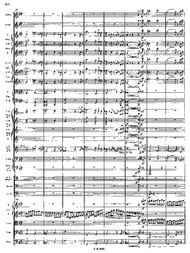
105 97

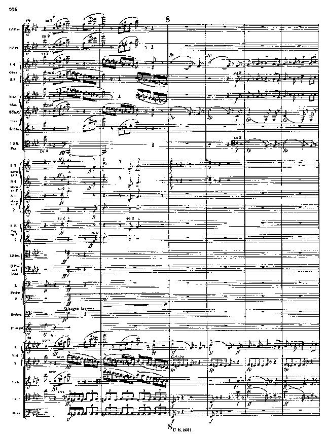
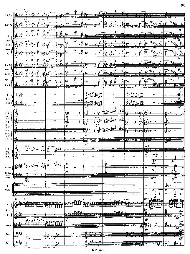
106 9

107 Table I.. Excerpt limits of anechoic recordings Excerpt no. ower limit Upper limit ength [samples] ength [s] Excerpt no. ower limit Upper limit ength [samples] ength [s]

108 Table I.. Excerpt limits of recordings in MGE Excerpt no. ower limit Upper limit ength [samples] ength [s] Excerpt no. ower limit Upper limit ength [samples] ength [s]

109 Table I.3. Excerpt limits of recordings in VTM Excerpt no. ower limit Upper limit ength [samples] ength [s] Excerpt no. ower limit Upper limit ength [samples] ength [s]

110 Table I.. Excerpt limits of recordings in PDB Excerpt no. ower limit Upper limit ength [samples] ength [s] Excerpt no. ower limit Upper limit ength [samples] ength [s]

111 !""#$%*)F)+)93'G)("##%)#---)"#-)H!:9!)-#'-%#- Table J.. Clock speed error per TASCAM recorder relative to TASC Instrument Brand Type Serial no. Clock speed error relative to TASC [ppm] TASC TASCAM D TASC TASCAM D TASC3 TASCAM D TASC TASCAM D TASC TASCAM D TASC TASCAM D TASC7 TASCAM D TASC TASCAM D TASC9 TASCAM D TASC TASCAM D

112 Table K.. Acoustic conditions for the ST early,d (f, d) = a * log (d) + b, obtained from I s on occupied stages, based on 3(source) * (receiver) = S-combinations. MGE (Wenmaekers Hak, a submitted). Frequency MGE VTM PDB a b a b a b ST Early,d [db] ST Early,d [db] ST Early,d [db] - - MGE - VTM PDB Hz S distance [m] Hz khz S distance [m] S distance [m] MGE VTM PDB MGE VTM PDB ST Early,d [db] ST Early,d [db] ST Early,d [db] Hz khz S distance [m] S distance [m] MGE VTM PDB MGE VTM PDB khz S distance [m] MGE VTM PDB

113 ST Early,d [db] khz S distance [m] MGE VTM PDB Table K.. Acoustic conditions for the ST late,d (f) as a fixed number, obtained from I s on occupied stages, based on 3*= S-combinations (Wenmaekers Hak, in press). Note that ST late,d is not dependent on S-distance (Wenmaekers Hak, b). Frequency MGE VTM PDB ST ate,d [db] MGE VTM PDB Frequency [Hz]

114 Nicolai - The influence of stage acoustics on sound exposure of symphony orchestra musicians Appendices part

115 Appendix - Measurement resuls Mahler piece per excerpt

116 eq 9 st violin eq MGE VTM PDB direct,own 3 3 ID ID Excerpt number [-] eq 9 nd violin eq MGE VTM PDB direct,own 3 3 ID ID Excerpt number [-]

117 eq 9 viola eq 3 3 MGE VTM PDB direct,own 9 ID 3 3 ID Excerpt number [-] eq 9 violin cello eq ID MGE VTM PDB direct,own ID Excerpt number [-]

118 eq eq ID 9 7 double bass ID Excerpt number [-] MGE VTM PDB direct,own eq eq ID 9 french horn ID MGE VTM PDB direct,own Excerpt number [-]

119 eq 9 clarinet MGE VTM PDB direct,own eq ID ID Excerpt number [-] eq 9 bassoon MGE VTM PDB direct,own eq ID ID Excerpt number [-]

120 eq 9 oboe MGE VTM PDB direct,own eq ID ID Excerpt number [-] eq 9 trumpet eq ID - ID MGE VTM PDB direct,own Excerpt number [-]

121 Appendix M - Model vs. - solo scale experiment

122 MGE PDB VTM st Violins ID viola # violin cello # double bass # French horn # clarinet # bassoon #3 oboe #3 trumpet # st violins # nd violins # direct,own () S distance [m] ID ID 7 7 direct,own () S distance [m] ID - - viola # violin cello # double bass # French horn # clarinet # bassoon #3 oboe #3 trumpet # st violins # nd violins # ID 7 7 direct,own () S distance [m] ID - - viola # violin cello # double bass # French horn # clarinet # bassoon #3 oboe #3 trumpet # st violins # nd violins # nd Violins ID viola # violin cello # double bass # French horn # clarinet # bassoon #3 oboe #3 trumpet # st violins # nd violins # direct,own () S distance [m] ID ID viola # violin cello # double bass # French horn # clarinet # bassoon #3 oboe #3 trumpet # st violins # nd violins # direct,own () S distance [m] ID ID 7 7 direct,own () S distance [m] ID - - viola # violin cello # double bass # French horn # clarinet # bassoon #3 oboe #3 trumpet # st violins # nd violins # Viola ID viola # violin cello # double bass # French horn # clarinet # bassoon #3 oboe #3 trumpet # st violins # nd violins # direct,own () S distance [m] ID ID viola # violin cello # double bass # French horn # clarinet # bassoon #3 oboe #3 trumpet # st violins # nd violins # direct,own () S distance [m] ID ID viola # violin cello # double bass # French horn # clarinet # bassoon #3 oboe #3 trumpet # st violins # nd violins # direct,own () S distance [m] ID Appendix M - Model vs - solo scale experiment

123 MGE PDB VTM Violin cello No data ID 7 7 direct,own () S distance [m] ID - - st violins # nd violins # ID 7 7 direct,own () S distance [m] ID - - st violins # nd violins # Double bass ID viola # violin cello # double bass # French horn # clarinet # bassoon #3 oboe #3 trumpet # st violins # nd violins # direct,own () S distance [m] ID ID 7 viola # violin cello # double bass # French horn # clarinet # bassoon #3 oboe #3 trumpet # viola # violin cello # double bass # French horn # clarinet # bassoon #3 oboe #3 trumpet # st violins # nd violins # direct,own () S distance [m] ID ID viola # violin cello # double bass # French horn # clarinet # bassoon #3 oboe #3 trumpet # 7 7 direct,own () S distance [m] ID - - viola # violin cello # double bass # French horn # clarinet # bassoon #3 oboe #3 trumpet # st violins # nd violins # French horn ID viola # violin cello # double bass # French horn # clarinet # bassoon #3 oboe #3 trumpet # st violins # nd violins # direct,own () S distance [m] ID ID viola # violin cello # double bass # French horn # clarinet # bassoon #3 oboe #3 trumpet # st violins # nd violins # direct,own () S distance [m] ID ID viola # violin cello # double bass # French horn # clarinet # bassoon #3 oboe #3 trumpet # st violins # nd violins # direct,own () S distance [m] ID Appendix M - Model vs - solo scale experiment

124 MGE PDB VTM Clarinet ID viola # violin cello # double bass # French horn # clarinet # bassoon #3 oboe #3 trumpet # st violins # nd violins # direct,own () S distance [m] ID ID 7 7 direct,own () S distance [m] ID - - viola # violin cello # double bass # French horn # clarinet # bassoon #3 oboe #3 trumpet # st violins # nd violins # ID 7 7 direct,own () S distance [m] ID - - viola # violin cello # double bass # French horn # clarinet # bassoon #3 oboe #3 trumpet # st violins # nd violins # Bassoon ID viola # violin cello # double bass # French horn # clarinet # bassoon #3 oboe #3 trumpet # st violins # nd violins # direct,own () S distance [m] ID ID viola # violin cello # double bass # French horn # clarinet # bassoon #3 oboe #3 trumpet # st violins # nd violins # direct,own () S distance [m] ID ID 7 7 direct,own () S distance [m] ID - - viola # violin cello # double bass # French horn # clarinet # bassoon #3 oboe #3 trumpet # st violins # nd violins # Oboe ID viola # violin cello # double bass # French horn # clarinet # bassoon #3 oboe #3 trumpet # st violins # nd violins # direct,own () S distance [m] ID ID viola # violin cello # double bass # French horn # clarinet # bassoon #3 oboe #3 trumpet # st violins # nd violins # direct,own () S distance [m] ID ID viola # violin cello # double bass # French horn # clarinet # bassoon #3 oboe #3 trumpet # st violins # nd violins # direct,own () S distance [m] ID Appendix M - Model vs - solo scale experiment

125 MGE PDB VTM Trumpet ID viola # violin cello # double bass # French horn # clarinet # bassoon #3 oboe #3 trumpet # st violins # nd violins # direct,own () S distance [m] ID ID viola # violin cello # double bass # French horn # clarinet # bassoon #3 oboe #3 trumpet # st violins # nd violins # direct,own () S distance [m] ID ID viola # violin cello # double bass # French horn # clarinet # bassoon #3 oboe #3 trumpet # st violins # nd violins # direct,own () S distance [m] ID Appendix M - Model vs - solo scale experiment

126 Appendix N - Model vs. - group scale experiment

127 MGE PDB VTM st Violins ID viola # violin cello # double bass # French horn # clarinet # bassoon #3 oboe #3 trumpet # st violins # nd violins # direct,own () S distance [m] ID ID 7 7 direct,own () S distance [m] ID - - viola # violin cello # double bass # French horn # clarinet # bassoon #3 oboe #3 trumpet # st violins # nd violins # ID 7 7 direct,own () S distance [m] ID - - viola # violin cello # double bass # French horn # clarinet # bassoon #3 oboe #3 trumpet # st violins # nd violins # nd Violins ID viola # violin cello # double bass # French horn # clarinet # bassoon #3 oboe #3 trumpet # st violins # nd violins # direct,own () S distance [m] ID ID viola # violin cello # double bass # French horn # clarinet # bassoon #3 oboe #3 trumpet # st violins # nd violins # direct,own () S distance [m] ID ID 7 7 direct,own () S distance [m] ID - - viola # violin cello # double bass # French horn # clarinet # bassoon #3 oboe #3 trumpet # st violins # nd violins # Viola ID viola # violin cello # double bass # French horn # clarinet # bassoon #3 oboe #3 trumpet # st violins # nd violins # direct,own () S distance [m] ID ID viola # violin cello # double bass # French horn # clarinet # bassoon #3 oboe #3 trumpet # st violins # nd violins # direct,own () S distance [m] ID ID viola # violin cello # double bass # French horn # clarinet # bassoon #3 oboe #3 trumpet # st violins # nd violins # direct,own () S distance [m] ID Appendix N - Model vs - group scale experiment

128 MGE PDB VTM Violin cello No data ID 7 7 direct,own () S distance [m] ID - - st violins # nd violins # ID 7 7 direct,own () S distance [m] ID - - st violins # nd violins # Double bass ID viola # violin cello # double bass # French horn # clarinet # bassoon #3 oboe #3 trumpet # st violins # nd violins # direct,own () S distance [m] ID ID 7 viola # violin cello # double bass # French horn # clarinet # bassoon #3 oboe #3 trumpet # viola # violin cello # double bass # French horn # clarinet # bassoon #3 oboe #3 trumpet # st violins # nd violins # direct,own () S distance [m] ID ID viola # violin cello # double bass # French horn # clarinet # bassoon #3 oboe #3 trumpet # 7 7 direct,own () S distance [m] ID - - viola # violin cello # double bass # French horn # clarinet # bassoon #3 oboe #3 trumpet # st violins # nd violins # French horn ID viola # violin cello # double bass # French horn # clarinet # bassoon #3 oboe #3 trumpet # st violins # nd violins # direct,own () S distance [m] ID ID viola # violin cello # double bass # French horn # clarinet # bassoon #3 oboe #3 trumpet # st violins # nd violins # direct,own () S distance [m] ID ID viola # violin cello # double bass # French horn # clarinet # bassoon #3 oboe #3 trumpet # st violins # nd violins # direct,own () S distance [m] ID Appendix N - Model vs - group scale experiment

129 MGE PDB VTM Clarinet ID viola # violin cello # double bass # French horn # clarinet # bassoon #3 oboe #3 trumpet # st violins # nd violins # direct,own () S distance [m] ID ID 7 7 direct,own () S distance [m] ID - - viola # violin cello # double bass # French horn # clarinet # bassoon #3 oboe #3 trumpet # st violins # nd violins # ID 7 7 direct,own () S distance [m] ID - - viola # violin cello # double bass # French horn # clarinet # bassoon #3 oboe #3 trumpet # st violins # nd violins # Bassoon ID viola # violin cello # double bass # French horn # clarinet # bassoon #3 oboe #3 trumpet # st violins # nd violins # direct,own () S distance [m] ID ID viola # violin cello # double bass # French horn # clarinet # bassoon #3 oboe #3 trumpet # st violins # nd violins # direct,own () S distance [m] ID ID 7 7 direct,own () S distance [m] ID - - viola # violin cello # double bass # French horn # clarinet # bassoon #3 oboe #3 trumpet # st violins # nd violins # Oboe ID viola # violin cello # double bass # French horn # clarinet # bassoon #3 oboe #3 trumpet # st violins # nd violins # direct,own () S distance [m] ID ID viola # violin cello # double bass # French horn # clarinet # bassoon #3 oboe #3 trumpet # st violins # nd violins # direct,own () S distance [m] ID ID viola # violin cello # double bass # French horn # clarinet # bassoon #3 oboe #3 trumpet # st violins # nd violins # direct,own () S distance [m] ID Appendix N - Model vs - group scale experiment

130 MGE PDB VTM Trumpet ID viola # violin cello # double bass # French horn # clarinet # bassoon #3 oboe #3 trumpet # st violins # nd violins # direct,own () S distance [m] ID ID viola # violin cello # double bass # French horn # clarinet # bassoon #3 oboe #3 trumpet # st violins # nd violins # direct,own () S distance [m] ID ID viola # violin cello # double bass # French horn # clarinet # bassoon #3 oboe #3 trumpet # st violins # nd violins # direct,own () S distance [m] ID Appendix N - Model vs - group scale experiment

131 Appendix O - Model vs. - Mahler piece per excerpt

132 MGE PDB VTM st Violins ID ID Excerpt number [-] ID ID Excerpt number [-] ID ID Excerpt number [-] nd Violins ID ID Excerpt number [-] ID ID Excerpt number [-] ID ID Excerpt number [-] Viola ID ID ID ID ID ID Excerpt number [-] Excerpt number [-] Excerpt number [-] Appendix - Model vs - Mahler per excerpt

133 MGE PDB VTM Violin cello ID ID ID ID ID ID Excerpt number [-] Excerpt number [-] Excerpt number [-] Double bass ID ID ID ID ID ID Excerpt number [-] Excerpt number [-] Excerpt number [-] French horn ID ID ID ID ID ID Excerpt number [-] Excerpt number [-] Excerpt number [-] Appendix O - Model vs - Mahler per excerpt

134 MGE PDB VTM Clarinet ID ID ID ID ID ID Excerpt number [-] Excerpt number [-] Excerpt number [-] Bassoon ID ID ID ID ID ID Excerpt number [-] Excerpt number [-] Excerpt number [-] Oboe ID - ID ID - ID ID - ID Excerpt number [-] Excerpt number [-] Excerpt number [-] Appendix O - Model vs - Mahler per excerpt

135 MGE PDB VTM Trumpet ID ID ID ID ID ID Excerpt number [-] Excerpt number [-] Excerpt number [-] Appendix O - Model vs - Mahler per excerpt

136 Appendix P - Model vs. - frequency domain

137 MGE High strings ow strings Woodwinds Brass eq [db] eq [db] eq [db] eq [db] st violins # nd violins # viola # 7 violin cello # double bass # 7 clarinet # bassoon #3 oboe #3 7 French horn # trumpet # eq [db] eq [db] eq [db] eq [db] st violins # nd violins # viola # 7 violin cello # double bass # 7 clarinet # bassoon #3 oboe #3 7 French horn # trumpet # ID ID ID ID eq [db] eq [db] eq [db] eq [db] k k k k Frequency [Hz] k k k k Frequency [Hz] k k k k Frequency [Hz] k k k k Frequency [Hz] Appendix P - Model vs. - Frequency domain

138 PDB High strings ow strings Woodwinds Brass eq [db] eq [db] eq [db] eq [db] st violins # nd violins # viola # 7 violin cello # double bass # 7 clarinet # bassoon #3 oboe #3 7 French horn # trumpet # eq [db] eq [db] eq [db] eq [db] st violins # nd violins # viola # 7 violin cello # double bass # 7 clarinet # bassoon #3 oboe #3 7 French horn # trumpet # ID ID ID ID eq [db] eq [db] eq [db] eq [db] k k k k Frequency [Hz] k k k k Frequency [Hz] k k k k Frequency [Hz] k k k k Frequency [Hz] Appendix P - Model vs. - Frequency domain

139 VTM High strings ow strings Woodwinds Brass eq [db] eq [db] eq [db] eq [db] st violins # nd violins # viola # 7 violin cello # double bass # 7 clarinet # bassoon #3 oboe #3 7 French horn # trumpet # eq [db] eq [db] eq [db] eq [db] st violins # nd violins # viola # 7 violin cello # double bass # 7 clarinet # bassoon #3 oboe #3 7 French horn # trumpet # ID ID ID ID eq [db] eq [db] eq [db] eq [db] k k k k Frequency [Hz] k k k k Frequency [Hz] k k k k Frequency [Hz] k k k k Frequency [Hz] Appendix P - Model vs. - Frequency domain

140 Appendix Q - Mahler studies - right ear in MGE

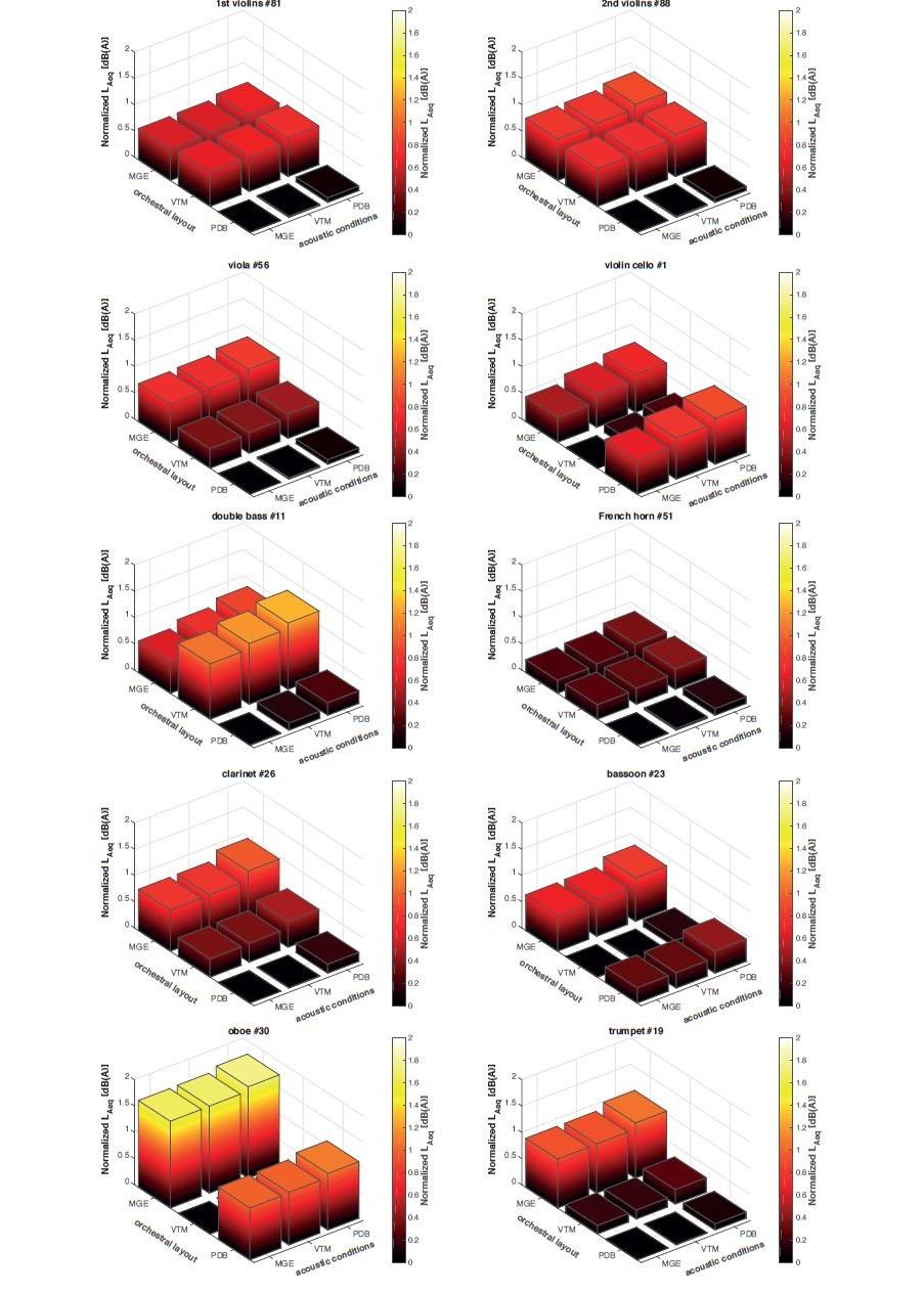
141