Operational Manual for Acoustic Measurements

Transcription

1 Apple ios Devices and Studio Six AudioTools Software Apple ios Devices and Studio Six AudioTools Software Operational Manual for Acoustic Measurements AudioTools 10x, SPLGraph 6x Revision 7.2: July 2017 Noise Measurement Services Pty Ltd

2 Contact: AcoustarWHS ph Brisbane web: July Acoustar and Noise Measurement Services Pty Ltd is a registered training organization (RTO Registration Identifier Code 41013), ABN Noise Measurement Services Pty Ltd is the Copyright holder for this Study Guide, with the exception of identified authored material. The copyright of acknowledged material remains with the identified author. Acoustar students are permitted to retain printed and electronic copies of this Study Guide for reference purposes. Acoustar is a Registered Trade Mark (No ). The trademark is registered in Class 41 Vocational education and Class 42 Scientific and technological services. Noise Measurement Services Pty Ltd is the owner of the trade mark. Acoustar Pty Ltd uses the name and trade mark under license. Disclaimer: This Acoustar Study Guide is prepared to meet the requirements of MSS025008A Monitor and Evaluate Noise and is based on the learning objectives, outcomes and limitations as may be stated in the Unit Descriptor. The Study Guide presents only the information that Noise Measurement Services Pty Ltd believes, in its professional opinion, is relevant and necessary to describe the issues involved. The Study Guide is subject to regular review. It is not a textbook and does not represent to address all issues relating to any particular topic. Students may freely use the material presented, but the intellectual property of the material remains with Studio Six Digital. 2 P a g e

3 Contents This Manual... 5 Device Compatibility... 5 Built-In Microphones... 5 Installing AudioTools... 5 Apps and Microphones for Sound Level Measurements... 6 STUDIO SIX DIGITAL APPS... 7 SPL Pro... 8 SPL Graph Audio File Analysis Quick-start for SPLGraph Setting up an iphone for Noise Logging Guided Access Mode SCHEDULER SPL Traffic Light Dosimeter RTA FFT Smaart Tools Impulse Response ETC - Energy Time Curve Room Treatment Generator Recorder Saving Data, Exporting, and Importing Save to Photo Roll Using Audio Files as Input Calibration Using Microphone Calibration Files icloud Support Dropbox Support Reference Curves AudioTools Wireless Transmission Loss Operation P a g e

4 Settings Sending Room Levels Receiving Room Levels Receiving Room RT Time Ambient Noise Levels Save / Recall Saving and Recalling Level Tests Saving and Recalling RT Results Saving and Recalling Results Gated Noise RT LARSA Transfer Function STIPA PRO ACU AUDIO COVERAGE UNIFORMITY TECHNICAL APP NOTES db vs. db Understanding SPL Measurements Headset Connected Microphones Audio Output itestmic Information iprecisionmic Sound Analysis System iaudiointerface Technical Information Terminology and Glossary Revision History Revision Date Change Author Drafting of core document to SSD and practice notes SSD, BT 4.1 Jan 17 includes draft application Transmission Loss and application Gated Noise SSD, BT 4.2 Feb 17 update SPL Pro; update itestmic; calibration and notes to various apps; BT PSEM notes removed 5.0 March 17 Dosimeter added to AudioTools SSD, BT 5.1 March 17 Update to SPL Pro and SPLGraph settings BT 5.2 March 17 Update to FFT ref AT SSD, BT 5.3; 5.4 April 2017 Update: Using audio files as input to Smaart, etc SSD, BT 6.0 April 2017 Updated by including LARSA, STIPA and Transfer Function SSD, BT 7.0 April 2017 Updated to include Audio Coverage Uniformity SSD, BT 7.1 May 2017 Updated with Scheduler; minor reformat to section headings SSD, BT 7.2 July 2017 Included hardware application and calibration documents SSD, BT 4 P a g e

5 This Manual Studio Six has developed a very wide range of apps for use in acoustics, design and placement of speakers, and technical assistance (e.g. signal generators, transfer functions, design tools and calculators). Not all of these apps are described in this guideline, as we (Noise Measurement Services) are concentrating on the acoustics applications. Note: the expressions we and the occasionally in the text refers to the authors of this Manual, Studio Six Digital. Illustrations in the text are from screenshots from an ipad or iphone apps may display slightly differently between the two. The text for this Manual is drawn directly from the Studio Six Digital website and it is recommended that the reader visit the website and YouTube on a regular basis to check the blog and FAQ updates: YouTube - Audiotools app or StudioSixDigital Device Compatibility AudioTools is compatible with most ios devices but better performance is achieved with iphone 5 and later devices. Built-In Microphones All of these devices include built-in microphones. These mics tend to be very consistent from one unit to the next, and are wide-range. However, Apple does include a very steep high-pass filter (which cuts low frequencies), presumably as a wind and pop filter. The low-frequency roll-off for the internal mic in these devices is very steep, on the order of 24dB / octave starting at 250Hz. However, with the advent of ios 6, and AudioTools 4.7, the low-frequency roll off filter is able to be turned off, thereby resulting in fairly flat response. Of these this is still basically a cell phone mic, and the performance is limited. Also, often it is found that real-world mics get dirty or damaged in usage and performance degrades over time. Studio Six Digital strongly recommends upgrading to at least ios 8, and the most current AudioTools release. Installing AudioTools To install AudioTools on one of the compatible devices listed above, simply search the App Store for AudioTools and purchase to install. Please note, some features require additional in-app purchasing. Access to an icloud account and gmail is very helpful for the saving of data. 5 P a g e

6 Apps and Microphones for Sound Level Measurements The following commentary is part of the Acoustar Noise Management training program. The Studio Six apps are very comprehensive in the functions that they make available to the user. As a minimum, these apps provide sound levels and sound character (octaves, third octaves, etc). For best results, however, an external microphone is needed. Apple ios System The Studio Six Digital apps tested by Acoustar for the noise monitoring training program include: AudioTools (full suite of applications) SPLGraph and SPL Graph Pro (all app options installed) Dual SPL Traffic Light FFT, RT60 and Transmission Loss Smaart Tools Photo: Apple iphone with SPLGraph app and external microphones. The microphones work with all the ios system apps. Microphone 1: Class 1 Larson Davis microphone, MicW phantom power preamplifier and two channel StudioSix interface module Microphone 2: Class 1 Aco Pacific microphone and StudioSix Class 1 preamplifier Microphone 3: Class 2 StudioSix itestmic microphone and preamplifier Microphone 4: Class 2 Dayton imm-6 headset microphone Microphone 5: Class 2 Acoustar Primo EM246 headset microphone 6 P a g e

7 STUDIO SIX DIGITAL APPS In this training guide we will be presenting apps that will be most often used in measuring environmental or workplace occupational noise. An external microphone is strongly recommended. 7 P a g e

8 SPL Pro SPL Pro is a professional-grade sound level meter for the iphone. It incorporates all the features of a dedicated SPL meter -- ANSI modes Slow, Fast, Impulse, Peak, and Leq, A and C weighting, Octave band filters, and the ability to be calibrated. See the SSD demo video for SPL Pro. This video was recorded on the simulator, within AudioTools. See the "db vs. db" section to understand what the SPL numbers mean, and why they might be different on different modules. SPL Pro conforms to all features of the ANSI and ISO standards for averaging sound level meters. To obtain this performance level, you will need to use SPL Pro with a suitable microphone, such as the itestmic or Precision microphone. How to Use SPL Pro Refer to the screen above. Mode SPL supports fthe standard ANSI decay times, and LEQ mode. All times are in terms of exponential decay, where the reading will decay by 20dB over the specified time. SLOW -- this mode uses a 1-second decay time. Good for getting a general reading of the ambient sound level. FAST -- this mode uses a 125ms decay time. IMPULSE -- not used very much, normally Peak mode would be used. This mode has a 35ms decay time. PEAK -- Peak mode show the peak value received since the last screen update. 8 P a g e

9 LEQ LEQ is essentially average SPL over time. This mode does an equal-weighted time average of the incoming SPL level. A timer shows how long the Leq has been running. Touch Reset to start the averaging over from the start. Tap Reset to begin a new LEQ capture sequence. The cumulative SPL level will be displayed. Filter You can select unweighted, which is wide-band; all frequencies are represented equally. A-weighting rolls off lows and highs fairly severely, and can be compared to voice band. C-weighting rolls off lows and highs gently, and is sometimes thought of as music weighting. Octave Band filters, 31, 63, 125, 250, 500, 1k, 2k, 4k, 8k, and 16kHz. These are Type 1 ANSI filters that in effect isolate a single octave band. Often used for noise analysis, or to test masking signals. Capture Tap the Capture button to store the current SPL level as the baseline reference level. This will be used to compute the real-time deviation in db. Use this for seat-to-seat comparisons, or to see how the SPL is changing over time. Generator Tap the Sine icon to turn on the pink noise generator output. Output Turn this switch on to route the filtered input signal to the output. Input Source Most ios devices allow us to control the input gain of the microphone. For those devices, which include all iphones, you will see two gain ranges when you go to the Input Sources page. Select the appropriate range for the environment as follows: Low Range With the internal ios microphones, this will cover a range of approximately dba SPL. High Range This will extend the range to dba SPL. FILES: 2.0, L, C, R, LS, RS, Lfe, All These options select a 5.1 signal if the option is installed. Normal setting is P a g e

10 SPL Graph SPL Graph is a powerful sound level chart recorder and noise logging system for the iphone, ipad, and ipod Touch. It works by averaging the SPL for a period of time range from 0.1s to 15 minutes (Leq), applying an optional weighting filter or performing octave or 1/3 octave analysis, and plotting the sound level. You can optionally record the audio or video for the graph, send notifications based on preset limits, and even automatically graph results at the end of a test. We also plot the A, C, and unweighted (Z) SPL values along with the octave or 1/3 octave data. SPL Graph can be configured for continuous data logging, remote file saving or ing of data, Ln statistical measurements, event notification, and more. Check out the video demo of SPL Graph. SPL Graph can record up to 24 hours of 1-second resolution sound level data per file, and can be configured to auto-save and restart for continuous operation. The graph starts displaying a oneminute window, and as each minute is recorded, the graph re-scales automatically and adds another more time to show the data collected so far. 10 P a g e

11 You can upload the data and recorded audio files to the PC or Mac. The file format is.wav,.caf, which is a compressed Apple format, or M4A, which is a 10X compressed file format. You can convert a.caf it to a Windows-compatible file using a tool like AVS Audio Converter. Also see the app note on Setting up an iphone for Remote Noise Logging in this section. Octave and 1/3 Octave SPL Logging Starting with iphone 4S, SPL Graph has an option for adding an SPL Octave and 1/3 Octave Logging module. This allows recording the frequency spectrum at every point on the graph (typically every second, although it can be longer), as well as recording the average spectrum for the entire measurement. We also plot the A, C, and unweighted (Z) SPL values along with the octave or 1/3 octave data. Use the cursor to select any single data point on the screen and inspect the spectrum for that point. NOTE: iphone 4 and ipod touch 4 do not have enough processing power for this module, and so the module is not available on those devices. See the Octave Logging Demo Video. The Octave Band Logging option also allows you to pick any single octave or 1/3 octave band, or overall, A, or C weighting, for the main red curve. And, the filter option for this curve can be selected and viewed even after the measurement has been completed. To set up Octave Logging, go to the Setup page in SPL Graph, and purchase the Octave Band Logging option, by tapping the Info button that appears over the Octave Logging selector. Then, just select with Octave or 1/3 Octave Logging. The test will now run in that mode. Octave logging also enables the 3D plot of data vs frequency vs time. Tap the 3D to switch to 3D display, where you can rotate the plot, and when the test is complete, use a timeline control to show the plot as it looked at different times in the test. The octave and one-third octave band values are saved as unweighted Leq sound levels (LZeq) by default. The only time this is not true is when the A or C weighting is applied in RTA or FFT. 11 P a g e

12 Charging indicator The V on-screen is the voltage indicator. If the V is green the iphone has more than 80% charge. If orange, the iphone has less than 80% charge. If the + sign is showing, the iphone is charging. Graphics The graph starts with a one-minute window, and as a minute is recorded, the graph re-scales automatically and adds another minute to show the data collected so far. Tap the speaker" play button to play back the recorded audio, and use the cursor to scrub the audio location on the graph. Use this feature to listen to events that you can see on the graph. You can scroll and scale the graph vertically, in db, by using standard swipe and pinch gestures. You can also scroll and expand and contract the time axis using gestures. Zoom out to a full 24 hours, or zoom in to a single minute, showing second resolution. Double-tap the screen to zoom out to show the entire graph on the screen. The time scale grid changes dynamically, highlighting minutes, ten-minute, and hour lines as as it runs. As the graph runs, the overall LEQ (average SPL) for the entire time period is computed and displayed on the screen. 12 P a g e

13 Swiping across the graph brings up a cursor that displays the exact db level and time for any point on the graph. Ln Statistical Data Logging Ln statistics may be enabled on the setup page. When on, these values will be computed, on the overall data: LMax LMin L95 L90 L50 L10 L01 If Full Data Save is turned on, these values are also stored for each data point (1.0s to 15m) that is recorded. In octave band mode, you can selected any single value, such as Z, A, or C weighting, or one of the octave or 1/3 octave bands for Ln calculations. Ln is calculated at 0.1s resolution, which matches many traditional logging sound level meters. You can choose to insert a traditional Fast or Slow detector before the Ln calculations, to match the operation of legacy analog SLMs. Settings SPL Graph has many options and features that allow you to customize it for any application, including setting it up as a continuous noise logging system. 13 P a g e

14 Audio/Video Recording Settings SPL Graph can record up to 24 hours of audio or video, or it can be setup to only record events that exceed a preset threshold. When the threshold is reached, 10 seconds of audio before the event is recorded, and recording will continue for 10 seconds after event. Video will start at the event time and will extend 10 seconds past the end of the event. For audio, you can select uncompressed WAV files, compressed CAF files (4x smaller), or M4A mpeg files, which are 10x smaller than wave files. For video, you can choose between several sizes. These files will be named the same as the stored file, with numeric suffixes following the file name. Turn on Audio Monitor if you wish to listen to sounds being recorded. Note that this may cause feedback if you are using the internal mic. Since the audio is recorded with the full dynamic range of the input, it may be difficult to hear the sounds that were recorded. Turn up the Playback Volume boost to increase playback level without changing the db measurements. Time Limits and Resolution Resolution controls the amount of time that is averaged in each data point. This can be selected to match the situation or to match a noise standard. You can select from 0.1s (if octave logging is off) to 60m resolution. Using the Time Limits control you can allow SPL Graph to start immediately when you tap the microphone icon, or you can delay it by some time, lock it to even clock hours, or, with Time Sync, you can lock it to even multiples of the selected Resolution time. This allows you to run multiple copies of SPL Graph on different devices, and keep the data locked in time. Ln Statistical Data Select flat (Z), A, or C weighting for the Ln values (if you are running octave logging - otherwise the selected weighting is used), choose to place a Fast or Slow detector before the Ln calculations are made. You can choose to also store 50ms (20 times per second) data to another file. This will be named the same as the main data file, with the.txt extension. It contains ASCII tab-delimited data and can be opened in Excel. Note that more Ln values are stored to the file than are shown on the screen, for clarity of the display. 14 P a g e

15 Minimal Display This feature allows SPL Graph to function with all of the data logging options and features running, while presenting a simple interface to the end user. This will be a simple screen, with only a db reading, clock and nothing more. The background color of the screen will change depending on the limits set. You can select Fast, Slow, or an Leq time, as well as the db levels for the red, yellow, and green colors. Also, if you turn on the Main Screen switch, the db level will appear on top of the graph. Auto Save Settings To setup SPL Graph for data logging, first set a Run Limit on the main Setup page, so that the test will stop at a set time. This can be any convenient interval, up to 24 hours (1440 minutes). Then, tap the Autosave Setup button, and set the options that you would like. Turn on Autosave to enable saving of data at the end of the run (when the Run Limit time is reached). Then, if you want the results ed, turn this option on and enter an address. If a valid address is set, the results will be ed to that address at the end of the run. Note that if you are using icloud or Dropbox you probably don't need to also the results. 15 P a g e

16 To continuously save results, also turn on the Restart After Save switch. SPL Graph can save data automatically at the end of a timed run, restart another run for continuous operation, and even the results back to at the end of the run. You can also have a screen shot saved at this time and ed along with the test data XLS file. icloud and Dropbox support mean that the data files can also automatically appear in the icloud folder or Dropbox. Just enable icloud or Dropbox on the General-Settings page, and every time that a file is auto-saved the data will appear on the cloud, if the device has internet connectivity. If it is offline, the data will be stored locally and migrate to the cloud automatically the next time that you open the app with internet available. Auto Save can turn the ios device into a powerful Type 1 approved sound level monitor, when used with an appropriate microphone, such as iprecisionmic. Notification Settings SPL Graph can also automatically send out notifications of SPL overage events. You can define up to 3 addresses to receive the notification, the weighting, the LEQ time that the SPL level is exceeded for, and you can even limit the number of s sent to prevent being bombarded with s. Notifications make it easy to monitor remote SPL events. You can also to choose to turn on ios notifications. This will cause a notification to be shown locally on the ios device, even the if the app is running the background. This will also cause the notification to be sent to Apple Watch. Audio and Video Recording The audio is recorded 16-bit, 48k, mono, as an uncompressed WAV file, or as a compressed CAF file using Apple s 4-to-1 IMA4 compression algorithm, or as an mpeg file using 10-to-1 compression. The storage requirements are shown here for 1 hour of audio: WAV file, uncompressed, 345mb/hr, 8.2gb/day CAF file, Apple compression, 86mb/hr, 2.1gb/dat M4A file, mpeg compression, 34mb/hr, 0.8gb/day 16 P a g e

17 To free up space, you can always delete the graph and audio or video files from the Save / Recall page. File Saving If you exit the app, or are interrupted with a phone call, the graph data will not be lost. SPL Graph will automatically save the graph, and reload it when you next open the program. You can also save a graph and the XLS data on the ios device, so that you can recall the graph later. We also support Dropbox, so that data can be sent automatically to the Dropbox when the file is saved. SPL Graph supports saving an unlimited number graphs directly on the ios device. You can recall these graphs and bring them up on the screen, and listen to the sounds that were made while the graph was recorded. You can also store an image of the screen to the photo roll. You can control the amount of data that you want stored by using the Full Data Save option on the main settings page. If this is turned off, you will only get a summary of the data. If you turn it on, you will get all the details for each data point. Use SMPTE Pink Noise\n\n Turning this on enables the use of SMPTE standard pink noise. See SMPTE for more information. If this is off, standard pink noise is used with a linear filter applied to white noise \n\n Allow Mixing Audio with Other Apps\n\n. Turning this on will let audio that is playing from another app, such as the music player, to continue playing while the app is running. If this is off, the audio from the other app will stop as soon as the app starts running. Microphone Calibration The microphone (internal, headset or lightning port) calibration is set in the Microphone Setup Tab. File Storage and Audio Settings File storage and audio settings are found under the General tab. 17 P a g e

18 See the Info page for an explanation of ios Gain, High Gain Override and Allow Mixing Audio with Other Apps Audio File Analysis Audio file processing is available for files created in SPLGraph in the Audio Tools app. (That is, not in the SPLGraph standalone app). The processing is available in FFT, RTA and Smaart. The audio file must be recorded in wave format (not CAF or m4a) and saved to icloud. The file can then be recovered and opened for processing. Open FFT and tap the spanner on the bottom of the page. This takes you to the FFT Setup page. Tap Input Source. This will take you to the Input Source page. Tap Select Input File on the bottom and choose the file. It will now process in the Main Screen, looping, playing just as it was recorded. The slider can be used to change the file position. 18 P a g e

19 Quick-start for SPLGraph The following sets up the app in a simple format to save Leq, Ln, and one-third octave data every second for 10 minutes. Audio and video are not saved using these settings. Tap and open the SPLGraph app Tap the SPOKE emblem, top left corner of the screen to open the SETTINGS page Tap GENERAL Tap CLOUD FILE STORAGE and choose icloud Tap Move Local Files to icloud and tap Done to return to the General screen Leave all the other General Settings in their default condition. Tap Done. The app is now back on the Settings page. If you are using the internal microphone tap Done. This returns to the main screen. Tap the SPANNER symbol at the bottom-right of the screen to open the SPL GRAPH SETUP page. Audio/Visual Set the Audio/Video Capture function to None Time Limits Set the Time Limits to Start Now Leave the Delay at none Set the Run Limit to 10 minutes: tap and type 00:10:00 Octave Logging Tap Full data Save to On that is, move the button to the right so it shows green Tap the 1/3 option Ln Tap the Compute button to green and tap to choose and accept A and Fast Resolution Tap and save 1s and choose Sec Minimal Display Leave in the default settings and tap Done top-left of screen Tap Auto Save Setup just above the Ln screen Record your addresses as requested Set all the options ON ; that is, move the button right to green Data is now stored and ed every 10 minutes to your address Tap done to return to the SPL Graph Setup screen Tap Notifications Enter your address and move Enable button to green. Set the SPL Weighting to A weighted Tap Done to return to the SPL Graph Setup screen and Done to return to the main screen. Main screen Tap the weighting selection bottom left of the screen to A Weighted Tap the microphone symbol. SPL Graph is now running and the chart will update every second for the next 10 minutes. Data storage is continuous until the app is stopped. 19 P a g e

20 Setting up an iphone for Noise Logging An iphone can be configured for unattended operation, to minimize and try to eliminate all interruptions that could stop a test in progress. If you do all of the below steps, you should have a solid iphone that won't do anything other than run the app. Prevent Interruptions Turn off all Notifications Settings->Notifications For each app listed, select the app and turn off Allow Notifications. Turn off Amber Alerts Settings->Notifications Scroll all the way to the bottom of the page and turn off both AMBER Alerts and Emergency Alerts. Turn off Background App Refresh Settings->General->Background App Refresh Turn them all off. Turn off all Automatic Updates Settings->iTunes & App Store Turn them all off. Forward Calls on the Phone Settings->Phone->Call Forwarding Turn this on, and enter any phone number. This will ensure that in case a wrong number tries to call the phone, it won't ever ring. Turn on Do Not Disturb Settings->Do Not Disturb Turn on Manual. Turn off Repeated Calls. Set Allow Calls From to No One. Set SILENCE: to Always. Turn Siri Off General->Siri We don't want Siri listening waiting to do anything. Turn Off Handoff General->Handoff & Suggested Apps Turn Handoff off. Turn Off Messages and Facetime Settings->Messages, Settings->Facetime Turn these off. Other Settings Enable Turn on icloud Drive, Keychain, and Find My Phone. You don't need an account or backups. Settings->iCloud We also need location services to be turned on, and microphone access. 20 P a g e

21 Settings->Privacy->Microphone and Settings->Privacy->Location Services 21 P a g e

22 Guided Access Mode Apple supports a mode that allows you to lock your ios device into running one app, that cannot be interrupted. This is called Guided Access. With Guided Access, you can make your ios device into a dedicated hardware device that is running one specific app. Guided Access always prevents things like operating system update notifications and running other apps, so we recommend that it always be used when running something like SPL Graph or Dual SPL Traffic Light for long periods of time, where you leave the ios device unattended, or it is running any test that you don't want interrupted. There are several options available, including ones that prevent the wake/sleep button from operating, so that the device can't be powered off, and even one that disables all touch GUI operations or just parts of the screen. Also, see our information about Setting up an ios device for Noise Logging for more tips about preventing interruptions. Setting up Guided Access Guided Access is a feature of ios, so some of the options may change from time to time. We are documenting its usage in ios 9. See the Apple documentation for more detailed information about Guided Access. To enable Guided Access, open the ios Settings app, and go to the General->Accessibility- >Accessibility Shortcut page. Turn off any options other than Guided Access. This will simplify bringing up the Guided Access options later. Now go back to the General->Accessibility->Guided Access page and turn on Guided Access and the Accessibility Shortcut. Also set a passcode so that you can totally lock out other users. This can be a different passcode than the device passcode. 22 P a g e

23 Using Guided Access With An App Now you are ready to start using Guided Access. Exit Settings, and open the app that you want to run. In this example, we are using SPL Graph. Triple-click the home button to begin Guided Access mode for this app. You will see a notification appear briefly saying "Guided Access Started". Now, triple-click the home button again and enter your passcode to bring up the Guided Access options page. It looks like this: You can exit Guided Access mode by tapping End, or go back by tapping Resume. Note that you can disable only parts of the screen if you like. In this example, I'm disabling access to the Toolbar and the Settings icon. Tap the Options button to bring up this page, where you can select what you want or do want to be enabled. Note that I have left the Sleep/Wake button active. Even in this case, you can't shut the device off, but you can put the app into the background. Turn off Touch if you don't want anyone who does not know the Guided Access passcode to be able to start or end the test. Tap Done to get back to the running app. 23 P a g e

24 SCHEDULER Scheduler is a powerful feature that allows you to create a test schedule that includes a number of audio and acoustic measurements that run sequentially, automatically. You can control the length of time that each task runs, whether the generator is turned on, how long to wait between tasks, or whether each task is started manually. Results are stored as each test completes, using a common naming format, so that you can go back and collect the results from the test. Using the Task Scheduler Scheduler is located under the Settings Menu. The Scheduler can be used to set up a group of tests to be run sequentially, automatically. Results are stored at the end of each test using a common file name convention. Scheduler cannot run every AudioTools module. For one thing, the module must be able to store data. Also, some modules require hardware interaction, and are not suitable for automatic test runs. In this document, we will call a "test" a complete test run, which may include many individual audio measurements, which we will call "tasks. Tasks are the modules that can run under Scheduler: SPL Pro SPL Graph RTA FFT ETC Smaart Amplitude Sweep Speaker Polarity Speaker Distortion STIPA Pro Recorder The Scheduler Screen When you first enter the Scheduler, you will see the main Scheduler screen. Tests are stored in files, in the public/test folder on the ios device, and on your Dropbox, if you have it linked. Each test file contains information about the test, and a list of tasks to run. The test files present are shown in a table on the Scheduler screen. You can add tests with the + button, delete a test by swiping across it, edit a test by tapping the "i" or arrow disclosure button, or tap on the test table cell to start the test running. After tapping the "+" button to create a new test, or tapping the disclosure button, you can edit the test file. 24 P a g e

25 Editing a Test To create a new test schedule, tap the + on the Scheduler screen. This will bring up the Test screen. The Test These are the parameters fro the Test: Test Name To change the name of the test, just edit the text field on the top of the Test screen. A new test will be created using the new name, and the old test (if already saved) will not be changed or deleted. Start Delay Set an optional time to wait before the test begins. This allows you to move the ios device, or to setup the testing environment before the test run starts. Time is shown in minutes and seconds. Time Between Tests Set an optional time to wait in between each task. This can allow time for the room to quiet down between tasks, for example. Time is shown in minutes and seconds. Prompt for Next Test Normally, each task starts automatically, after the Time Between Tests. Turning this option on allows you to control when the next task will start manually. The Scheduler will wait for you to tap a button before it continues on to the next task. Lockout Local Control When a task is running, you can interact with the screen, which could affect the outcome of the measurement results. Turning on this option ensures that the task will run undisturbed. Note: It is possible to create a scenario where a task is running, and you can't interrupt it, for example by setting a very long task run time with lockout turned on. The only way to exit the app would be by force-quitting it. To do this, double-click the menu button, and follow the ios procedure for force-quitting an app, to end the app operation. Task List Below the test settings is the list of tasks. This list will be empty until you add a task, using the "+" button. You can also delete a task by swiping across the table cell, or reorder the tasks after tapping the Edit button and moving them by touching the control on the right and dragging the cell to a new position in the list. After you tap the "+" button, or when you tap the task table cell, the Task editing screen appears. The Automated Task The test consists of a list of tasks that run in sequence. You can have as many tasks as you wish, but note that if the same task runs twice in a given test run, the last task run will overwrite any previous task data files (except in the case of the surround signal generator, see below). 25 P a g e

26 Task Parameters The individual task settings, such as octave banding, weightings, decay times, and graph parameters are all set locally in the module. These settings are automatically saved, and will be in effect when the automated task runs. Make sure your tasks are setup the way that you want them before you start the test schedule. The run time parameters for the task are set on the Task Screen. These include the length of time that the task will run, whether it will turn on the generator, and the task itself. Generator Set up the generator for this task using the Generator panel. You can turn on the generator, select the signal type, and for sine or square waves, the frequency. You can also select the balanced / mono signal mode. Note that some tasks, such as STIPA, will always use their special signal. You still have to turn on the generator switch if you want the signal to play. Surround Signals Surround signals may be selected, if you have the Surround Generator module unlocked. When a surround signal is selected, the channel designator will be added to the file, just before the date, so that you can run a number of surround tests in the same test run without the files overwriting. Run Time Set the time that you wish the task to run in this field. Note that you will have to take into account any special considerations for the actual task. For example, if the Amplitude Sweep module is set to run a 30 second sweep, make sure you allow enough task run time for the sweep to complete. The same thing applies to STIPA, which requires a certain test length to complete. Select Task Select the task from the list of available tasks. If a measurement is not included in this list, it is not supported for automated tests 26 P a g e

27 SPL Traffic Light SPL Traffic Light is available in two formats: as a dual-display and as single display. The app is a SPL monitor, designed to be used to monitor SPL levels for live concert sound, community noise, and any public space that needs to be in compliance with sound level regulations. Use SPL Traffic Light with the built-in ios device microphone, or pair it with the itestmic for Class 2 results, or use it with the iprecisionmic for Class 1 performance. Note that it is possible to certify the entire instrument as Class 1, by sending iprecisionmic and the ios device to an independent testing lab. Having two sound level monitors allows SPL Traffic Light to adapt to nearly any community noise standard regulation, since you can set one meter for C weighted Fast, and the other for an Leq (average) time. The example here shows exactly that setup. This flexibility makes the SPL Traffic Light the most versatile SPL monitoring system available on any platform. The top control selects which SPL monitor the settings apply to. Enter the db trigger levels for the three colors, and select the weighting or octave band. You can also enable notifications, based on the display criteria for the red db trigger level. Notifications can be based on just one SPL monitor triggering into the red zone, or either or both triggering. Enter the own gmail credentials for the notification server. Note that Google's policies may require you to go to the own gmail settings, and enable access from a third party app. Set the three color trigger db levels, dynamic response, and weighting seperately for each SPL monitor. 27 P a g e

28 See the Traffic Light videos for the single and dual displays at: 28 P a g e

29 Dosimeter Dosimeter is a dual-display and single display SPL monitor, designed to be used to monitor SPL levels for live concert sound, workplace noise, and any occupational noise activityt that needs to be in compliance with sound level regulations. Use SPL Traffic Light with the built-in ios device microphone, or pair it an itestmic or iprecisionmic. Dosimeter applies the following noise criteria: ISO OSHA HC OSHA PEL NIOSH TWA ISO 1999:2013 is currently the internationally accepted standard for calculating noise exposure and risk of hearing impairment. The ISO standard applies a 3 db exchange rate, no time weighting (i.e. LAeq is applied), no threshold and a criterion level of 85 db OSHA Hearing Conservation applies a 5 db exchange rate, the use of a Slow time weighting, an 80dB threshold and a criterion level of 90 db OSHA Permissible Exposure Level applies a 5 db exchange rate, the use of a Slow time weighting, a 90dB threshold and a criterion level of 90 db National Institute for Occupational Safety and Health (NIOSH) recommends the use of a 3dB exchange rate, the use of a Slow time weighting, an 80dB threshold and a criterion level of 85 db Time weighted average the sound levels are calculated over 8-hours for 100% dose In addition, the sound level meter function can measure C-weighted peak values in a one-minute interval. An excellent summary of the application of different noise exposure metrics is provided in: Tingay J. & Robinson D. A practical comparison of occupational noise standards. Inter.noise P a g e

30 30 P a g e

31 31 P a g e

32 RTA RTA is a full-featured filter-based one-third octave Real Time Analyzer. *** NEW: Check out the new demo video of RTA. How to Use RTA Here is the RTA main screen: 32 P a g e

33 Band Size To use RTA, select the band size that you want, either Octave or 1/3 Octave. The octave and onethird octave band values are saved as unweighted Leq sound levels (LZeq) by default. The only time this is not true is when the A or C weighting is applied in RTA or FFT. Decay Modes and Speed Select the decay mode and speed. You can select one of the exponential decay modes, which are labelled in seconds. The seconds indicate the amount of time for a bar to decay by 20dB. Also, you can select Peak Hold, which holds the highest value that a bar has reached. To reset Peak Hold, re-select Peak Hold mode. There is one more mode, Average. This mode performs a continuous equal-weighted average, from the time you start the RTA with the Play button in this mode, until you Pause the RTA. Even then, you can continue the average by pressing Play. To reset Average mode, tap the Reset button on the screen. Play / Pause Touch the Play/Pause icon to begin. Anytime one of the parameters is changed, the RTA will revert to Pause so that the new parameters can be in effect for the most accurate readings. Screen Scaling & Resolution Once the graph is running, you can adjust the screen db scale by sliding the graph and up and down. You can also change the db resolution showing on the screen by pinching -- pinch together to get more db on the screen, or pinch apart to get less vertical db, and thus more detailed resolution. Double-tap the screen to auto-fit the graph to the display. You can turn on Lock Graph Scale if you want to set a graph range and not have it change on the main screen. The level may still be panned up and down, but the range will not change and the double-tap will not change the scale or range. Saving a Screen Image You can take a snapshot of the screen by touching the Save Image button. The image will be saved in the photo roll, and can be ed or transferred to the computer using various third party apps. Noise Curve Overlays To display a noise curve overlay, flip the screen over by touching the info icon in the navigation bar, and select one of the overlays: NCB -- Balanced Noise Curve, RC -- Room Curve, PNC, NR, or Noise Rating, used in the EU, and the cinema large-room X-curve. The overlay will appear on the graph. To read the noise curve value, find the lowest curve that does not have any bars touching it. You can interpolate between curves to estimate an exact curve number. Now see the overall noise overlay curve value -- in octave mode only, since the noise curve values are only defined for octave band mode. 33 P a g e

34 Graph Weighting You can select none, A, or C weighting. None will show the actual level of each bar. If you select a weighting, the bars will show the weighted equivalent. This means that the lower frequencies will show lower values in A or C weighting. Max / Min Bars You can turn on this option on the setup page. When active, the maximum and minimum levels of each bar is stored, and shown as blue and green bars on the screen. To reset the bars, just double-tap the screen. Peak Decay Bars Peak decay bars will show you the actual peak level of the band, no matter what decay mode you have selected. They automatically decay and will drop into the graph when there is no level above the bar. Hearing Threshold Line This line shows the approximate level below which sounds are inaudible to the human ear. This varies somewhat by person, but even so it can be used as a guide to when sounds are not audible. Overall SPL The overall unweighted db SPL level is shown just above the graph, on the right side. Choose unweighted SPL, or A or C weighting on the setup screen. Audio Monitor Turn this on to listen to the incoming audio signal in the output. Note that this may cause feedback. Turning on the generator disables Audio Monitor. Pink Noise RTA includes a full-featured signal generator, which includes sine waves, square waves, white noise, and pink noise. Pink noise has equal energy in each octave (or 1/3 octave), so in theory if the system is flat, you will see a flat line on the RTA display. Room Tuning In practice, the RTA is really showing the sum of the direct sound as well as the reflections, so this is not 100% correct. Also, most people roll off the high end somewhat, and many like to boost the low end. So, use the RTA and it's information, but also use common sense, and don't make extreme EQ changes. You're usually better off making conservative changes in EQ, but you should definitely try moving speakers and subs around, and watch the effect in the RTA. Here are some links to learning the basics on room tuning with an RTA: _using_rta_fft P a g e

35 FFT FFT is a high-resolution audio analysis tool available as an in-app purchase in AudioTools. It uses the Fast Fourier Transform (see below) to analyze incoming audio, and displays a very detailed graph of amplitude vs. frequency. FFT showing full frequency range: FFT showing low-frequency analysis range: 35 P a g e

36 This application has been designed for acoustics work, and so the FFT bins have been normalized to octaves, to get a display that will show a flat line for pink noise. You can control both the level of graph smoothing and decay time, to get as much or as little detail as you require. FFT showing multiple recalled measurements, on iphone 5. Features: FFT size from 4096 to 32k (on newer ios devices) Difference mode to compare 2 graphs Peak frequency readout in real time Signal generator can generate sine waves, square waves, white noise, and pink noise. Cursor: Move the finger across the screen to get a cursor to read out exact db levels and frequencies Touch-GUI: use pinch gestures to scale the graph and zoom in on frequencies. Double-tap to normalize the graph to full range, and fit the entire graph on the screen. Both full range (20-20kHz) and low range (5Hz to 3100Hz) are available. Overall db display Save the graph image to the photo roll to include in a report Export the data in XLS format. FFT windowing available FFT Configuration Examples Analyze Speaker Response: Use Pink noise as the test signal, select Equal Points Per Octave, select 1/6 or 1/3 octave smoothing, select 1s Decay time. Music Analysis: Signal generator off, select the 2048-point FFT, 0.5s Decay, 1/24th octave smoothing. FFT Size Choose the size of the FFT on the setup screen. The larger the size of the FFT, the more resolution you will have, but the slower the response time. If you choose Equal Points Per Octave, each octave 36 P a g e

37 will have high resolution (equivalent to the upper half of a 512 point FFT), but the lower octaves will update much more slowly. Use this mode for steady-state sound inputs, such as pink noise. (See the section above for more information about FFT size). FFT Windowing When turned on, the data is windowed before sending it to the FFT. This has the effect of reducing noise artifacts, and allowing greater dynamic range on the FFT. With windowing turned on, you can get greater than 100dB of dynamic range when looking at sine wave signals. Operation Smoothing Select Octave, 1/3 octave, 1/6 octave, 1/12 octave, 1/24 octave, or none. Smoothing averages the FFT db values around each graph point logarithmically. Decay Mode The decay times apply to the graph db values. A decay time of one second will cause a point to decay at the rate of 20dB/second. Peak Hold holds the highest value received, and Average is a true linear average of all readings over the time of the average. To clear Peak or Average mode, select another mode momentarily and then go back to Peak or Average mode. NOTE: In EPPO mode, the decay time on the lower octaves is the same as the upper octaves, but since they are not being refreshed as often, the will jump up and then decay back down. Graph Scrolling The graph will scroll up and down when you slide one finger up and down on the screen. Use a two-finger vertical pinch to adjust the screen scale, to see more or less db on the screen. Use a horizontal open-pinch gesture to spread out the screen and zoom in on the frequency axis. When the frequency scale is zoomed, you can use two fingers to pan the graph horizontally. At any time, double-tap the screen to normalize it. This will show the full frequency range, and fit the graph to the screen. The state of the graph is stored as you make changes, so the next time that you start the FFT app, the zoom and scale settings are restored. Cursor Swiping left and right will bring up a cursor, which you can dismiss by swiping off the graph to the left. Generator Touch the sine wave icon to bring up the built-in generator. You can select the signal type, and for sine and square waves, the signal frequency. Note that digitally-produced square waves start to alias badly above about 2000 Hz, so you will get audio artifacts. The generator frequencies always change smoothly, to prevent zipper noise, and turn on and off with soft muting. 37 P a g e

38 Like the other calculations, the generator waveforms are created digitally using 64-bit floating point math, and are very accurate and low-distortion. Note that we have found that running the headphone output 1 click below maximum yields the lowest distortion waveforms. File Save and Recall Tap the folder button to access the AudioTools advanced and complete save/recall system. See the Save / Recall page for full details. Overall db Display The overall, unweighted SPL level is shown at all times on the screen in the upper right-hand corner. This is the same value that is shown on the calibration screen. Clipping If clipping of the input occurs, the words "Clipping Detected" will be displayed above the graph in the upper left-hand corner in red for 1.5 seconds. Octave and one-third octave band values The octave and one-third octave band values are saved as unweighted Leq sound levels (LZeq) by default. The only time this is not true is when the A or C weighting is applied in RTA or FFT. SETUP The March 2017 revision has additional features to the earlier (following) setup information. 38 P a g e

39 Let us take a quick tour of the FFT Analyser s Interface: 39 P a g e

40 40 P a g e

41 41 P a g e

42 42 P a g e

43 Windows for spectral analysis: 43 P a g e

44 Reference Curve FFT also includes support for the optional Reference Curves feature. The example above shows using a single reference curve, with a +/- db range to say whether or not the live curve is within that range. The green dot shows that this curve passes. Full Range / Low Frequency Mode Full Range shows 20-20kHz range, while Low Frequency mode shows 5Hz to 3100Hz. Audio Pass-Through Turn on or off to allow audio that is coming in to the unit to be presented at the output. Turning on the generator overrides audio-pass through. Difference Mode This switch turns difference mode on and off. When turned on, the most recently recalled graph (if any) is used as a baseline for the FFT function. In other words, the recalled graph is subtracted from the current FFT graph. You can use Difference Mode to compare speakers, or do a before and after comparison of an acoustic space. 44 P a g e

45 Peak Tracking Turns peak tracking on, showing the frequency either on the cursor, or in large text on the screen. The algorithm uses the actual highest FFT bin, and does not use the calibration compensation, so it may not be the highest point on the graph. Input Source This is the standard AudioTools input source selection screen, where you can choose microphone gain, or change settings. About the FFT Calculation FFT stands for Fast Fourier Transform, which is a mathematical algorithm that breaks a signal into frequency bins. Each bin is the same size, in Hertz. The size of the FFT determines the width of the bins in Hertz. Bin width = sample rate / FFT size. Since we are running at the iphone's maximum sample rate of samples/second, for a 1024 point FFT each frequency bin would be 48 Hz wide. This is gives us great resolution at 10kHz, but poor resolution at 32 Hz. We can run larger and larger FFTs, but since we first have to store up all the samples to fill the FFT, and then do the math, the lag time starts to increase and the display becomes less and less responsive. In FFT, we provide the choice of FFT size, currently from 4096 points to 16,384 points (32,576 on the newer ios models). In addition, we provide another mode, which we call Equal Points Per Octave (EPPO). In this mode, we run a fairly small FFT (currently 512 points), but we only use the top octave from this FFT. So, we get a resolution at 10kHz of about 93Hz. Another way to look at it is that we get about 120 data points in the top octave (think of it as 1/120th octave resolution, which is about right). Then, we decimate and filter to get the sample rate down to 24kHz, and then run another 512 point FFT. So again, we get 1/120th octave resolution. We continue this process right down to the lowest octave. The result is excellent resolution across the frequency spectrum. The cost is that each octave only updates half as quickly as the octave above it, so the low octaves update much more slowly. The upper octaves retain very quick response. EPPO is best used with steady-state signals, such as pink noise, or to analyze constant noise signals. If you want to see the entire graph updating quickly, use 4096 or 8192 points. Note that due to the fact that there are individual FFTs running for each octave, you may see graphical anomalies in the noise floor -- for example, since the decimation filter cuts off frequencies above the Nyquist frequency, the lower FFTs don't even get the higher frequencies, and so might have a lower noise floor than the upper FFTs. This is normal. You can adjust the graph to move the entire FFT noise floor off the bottom of the screen to get a cleaner looking graph. All calculations are done in 64-bit floating point for the best accuracy and to get the lowest possible noise floor. 45 P a g e

46 Smaart Tools Smaart Tools was developed by Studio Six Digital in collaboration with Rational Acoustics and is based on the proprietary algorithms, techniques, features & color mapping found in the Smaart v.7 acoustic test and measurement software. Smaart is a registered trademark of Rational Acoustics. The video can be found at: Transfer Function Studio Six Digital also offers Transfer Function, which is not derived from the transfer function in Smaart 7. It includes many powerful features, including magnitude, phase, and coherence graphs, and an impulse-response based sample-accurate delay finder. Transfer Function also now works with the internal ios mic, with the generator in loopback mode, so you can do testing for frequency response, phase, and delay using just an ios device. In this mode, you are limited to only using the internal pink noise test signal. The functions of the Transfer Function module and the Smaart Tools Single Channel module do not overlap, so they are offered for purchase separately. For one thing, Transfer Function requires a twochannel interface, while Smaart Tools Single Channel is a one-channel spectrum module, that works great with the built-in microphone. Smaart Tools Single-Channel Module The single-channel module includes the following features from Smaart v.7: the RTA Bar graph, RTA Line graph, RTA Bar & FFT graph, and the Spectrograph. On the iphone and ipod touch, there is an additional graph, the Spectrograph with the RTA Line graph on top of it. Here's a screen shot of that graph from iphone 4: 46 P a g e

47 All of the RTA banding options available in Smaart v.7 are available, including log, lin, Octave, 1/3rd, 1/6th, 1/12th, 1/24th and 1/48th Octave modes. The decay modes from Smaart v.7 are also available, and include None, 1, 2, 4, 8, and 16 averages, and the Smaart 1-10 second custom decay settings, as well as Infinite, Fast, and Slow. The frequency scale can be zoomed down to a single octave, and the db scale can be zoomed down to 1dB resolution. Double-tap the screen to return to full frequency response, and to auto-scale the db scale. Real-time Spectrograph history is saved, just swipe to see sound events that have scrolled off the screen. 47 P a g e

48 Other features include high-contrast mode, variable Spectrograph speed, vertical or horizontal running Spectrograph, Difference mode, Peak Tracking, and FFT Windowing. All of the standard AudioTools features, such as Save / Recall and the Generator Panel are available. All settings are automatically saved and restored the next time that you run the app. Because the processor on the iphone or ipad is not as powerful as a desktop machine, the number of updates per second is lower than a desktop or laptop machine. ipad2 however, with its faster processor and graphics, runs Smaart Tools at near native desktop speed. On ipad, split graph mode is available, so that you can put any two graphs on the screen at the same time. Here is a screen shot of the RTA Bar graph and the Spectrograph running on the ipad. (Image smaller than real size). 48 P a g e

49 49 P a g e

50 Impulse Response The Impulse Response module for AudioTools or standalone application provides an easy way to capture an IR audio file on ios devices, and also calculates the most-needed metrics from the data. Impulse Response is an ios port of a powerful mathematical model developed on desktop computers by Daniel Valente, Ph.D Architectural Acoustics, Rensselaer Polytechnic Institute. In seconds, a complete set of measurements is made that describe the acoustic character of a room, or the response of a loudspeaker. Impulse Response on the ios device will give you very good results, even with the built-in mic. Of course, you are limited to moderate SPL levels, and the lowest frequency bands will not be as accurate as when used with iaudiointerface2 or itestmic, but Impulse Response will give you accurate reverb decay times and other measurements. When you first access the Impulse Response recording screen, the reference sweep files will be downloaded. Or, you install them directly using itunes. This is especially useful if you are using the Surround Signal Generator. Be sure to check out our Impulse Response demo videos. Also see our two new videos, New Features in Impulse Response, and Gated Loudspeaker Measurements. The Impulse Response can be computed either from recording an actual impulse, like a balloon pop or handclap, or from recording a swept sine wave which is the converted to an impulse through deconvolution, all from within the iphone. Important: make sure you download our IR sweep files below, and play them from another ipod or a CD when recording an impulse response sweep. If you have not downloaded them in a while, please update to the latest versions on this page for best results. Recording an Impulse Response You can record either an actual impulse, or a swept sine wave that the app will deconvolve into an impulse. If you plan on recording a swept sine wave, download our three excitation signal files and burn them to a CD or put them on another ipod. 50 P a g e

51 You can also play the sweeps on another ios device with Remote Control Generator. Also, you can use AudioTools Wireless for remote recording of Impulse Response files. To record your impulse response, go to the Impulse Response module in AudioTools, and tap the sine wave icon, which will bring up the Recording screen. The first time that you access this screen, the three reference swept sine signal files will be downloaded from our server and saved on your device. You can always re-download them by tapping the "reload" button. This could become necessary if we change the sweep files in the future. Next, select the type of impulse response that you will be recording: Impulse, 3 second sweep, 7 second sweep, or 14 second sweep. Recording an Impulse To record an impulse, such as a handclap or balloon pop, just start recording, and create the impulse. Make sure that the Clip indicator does not appear. You can also listen to the impulse to check it, by pressing the Play button. When you are happy with the recorded impulse, tap Done to return to the calculations screen. After recording the impulse, tap Done to get back to the main screen, where you will see the ETC of the impulse. Recording a Swept Sine Wave 51 P a g e

52 You can select a 3 second, 7 second, or 14 second sweep. The tradeoff is that the shorter files process much more quickly, and require less device memory (although we have not yet found a situation where any device has actually run out of memory), and the longer files generally will give you better a better signal to noise ratio (S/N). You may want to start with a 3-second sweep as you get your setup working properly, and then switch to a longer file if you need to. Next, setup your playback system with the CD or ipod playlist that you created earlier. Connect to a system with only one speaker active, and try playing the sweep. Listen for obvious distortion or other problems. When you are ready to start recording, tap the Record button on the Recording screen, and then start the sweep playing. You will hear a short sync tone, followed 5 seconds later by the sweep. Wait until the minimum time displayed on the screen is reached before tapping Stop to end the recording. Watch the level meter as the sweep runs. Check that "Clip" does not appear on the screen, and that the sweep got more than half-way up the level meter. The yellow area is perfectly fine. If you like, you can play back the sweep and listen to it. At the end of the recording, a message box will appear asking whether you want to Deconvolve the sweep, or Cancel. If you are happy with the recording, choose Deconvolve. A series of calculations will begin, that make take up to several minutes, depending on the speed of your device. The new models are much faster. If all goes well, you will see the word "Done" in green, and you can tap Done and go on to the calculations screen. If there is a problem, it will be shown on the screen. The most likely problem is that the sync pulse may not be found. The sync pulse must occur at least one second after starting the recording, and must be within 20dB of the loudest part of the sweep. Also, the recording must be long enough to include at least 5 seconds of decay after the sweep. Normally, just waiting for the final sync pulse will allow enough time. When you go back to the calculations screen, the ETC will be computed and shown on the screen. From here you can look at other parameters and metrics, or trim (edit) the IR. Impulse Plot 52 P a g e

53 The Impulse plot shows the decay of the IR visually. You can use the cursor to read out the exact level magnitude and time. Also, you can tap the Play button to play the impulse. This can be useful to listen to the sound of a pulse decaying in the room, especially if you have created the impulse from a swept sine, by deconvolution. You can also use a pinch-zoom gesture to expand the image on the screen to see more detail. Editing the Impulse Response Often you can get better results by trimming the start and end of an impulse response. If you have recorded an actual impulse, it is highly recommended that you trim the result. If you have recorded a swept sine, sometimes the resulting IR will need some trimming before the impulse, and the noise after the decay curve can be trimmed to shorten the screen window for a better look at the data. Before editing IR When running a swept sine, if the sample rate of the playback device is slightly different than the sample rate of the device that the app is running on, even by just a few Hz, you may see a shorter false peak before the actual impulse. It is important to trim this for the best results. To edit an IR, go to the ETC screen, and use the pinch/zoom gesture to expand the display. Your goal is to remove extraneous sound before the actual impulse begins, without cutting into the impulse itself, and to remove noise after the decay ends, without cutting into the decay curve itself. The result needs to be at least 0.5 seconds long. 1.0 second is fine. 53 P a g e

54 After editing IR When you have trimmed the ETC, tap the Edit button and select Save File. This will remove the areas of the IR that are not on the screen and the ETC and cause calculations to be re-done. After trimming, you can then select one of these calculations to display in a bar chart, either by octave band or 1/3 octave band. Calculations are done as needed when you change graph selections. Windowing the IR In some cases you will get better calculation results by windowing the IR. Windowing can also be used to inspect a portion of the IR, and to remove reflections from the IR so that you can see the frequency response of a loudspeaker, without the effects of the room. The window is applied before all of the calculations are done, but is used most often in conjunction with the FFT plot, in order to inspect the frequency spectrum of a portion of the IR. Windowing is controlled by these parameters, which are accessed on the Setup page. Tap the wrench icon to bring up the Setup page. The left and right portions of the window are controlled separately, so that you can precisely control the window. There are controls here for the size of the left and right windows, and the reference time. Normally you will reference the window to 0.0 ms, which is the time of the peak of the IR. You may shift the windows if you wish to inspect the frequency spectrum at some point in the decay, for example to see the sonic coloring of the room as the signal decays. You can also select the function that shapes each window. Rectangular is a hard cut of all data before or after the window, but normally you will get a smoother FFT. 54 P a g e

55 Here is an example of a typical windowed IR, using the settings shown above. Note that we have windowed out the noise before the direct sound, and we have also windowed out most of the noise after the decay. This is a typical use of windowing to get better overall IR results. Windowing can also be used to inspect loudspeaker frequency response, independent of room effects. Octave and 1/3 Octave Bar Charts T20 -- T20 is the decay rate of the impulse response or reverberation time, the time that is takes for a sound to decay by 60 db in a space. By using a noise compensation technique to avoid inaccurate representations of reverberation time, the decay rate is calculated by determining the slope of the decay function from -5 db to -25 db, and extrapolating the time to a decay of 60 db. T30 -- T30 is the decay rate of the impulse response or reverberation time, the time that is takes for a sound to decay by 60 db in a space. By using a noise compensation technique to avoid inaccurate representations of reverberation time, the decay rate is calculated by determining the slope of the decay function from -5 db to -35 db, and extrapolating the time to a decay of 60 db. 55 P a g e

56 C50 The Clarity Factor (50ms), expressed in decibels, is the ratio of the early energy (0-50 ms) to the late reverberant energy (50-end of the decay of the IR). C50 is perceptually aligned with speech perception. C80 The Clarity Factor (80ms), expressed in decibels, is the ratio of the early energy (0-80 ms) to the late reverberant energy (80-end of the decay of the IR). C80 is perceptually aligned with music perception. 56 P a g e

57 EDT Early decay time represents the decay function of the IR in the slope of the early part of the energy decay curve. It is the slope of the curve limited from 0 db to -10 db extracted to a decay of 60 db below to stopping of the direct sound energy. EDT is typically associated with the perceived reverberation time in a room. CT - Center time or Ts is the time after the onset of the direct sound to the time where half of the energy has decayed in the IR. It is the time corresponding to the "balancing point" or center of gravity of the squared IR. Center time is correlated with reverberation time, so center time increases as a function of reverberation time. 57 P a g e

58 Definition Similar to the C50 metric, definition represents the ratio of sound arriving in the first 50 ms of the IR compared to the rest of the IR. It is expressed as a percentage and correlates to speech perception in a room S / N Signal-to-Noise ratio represents the difference between the measured signal captured by Impulse Response versus the noise floor present in the room under test. It is a good tool to verify that the measurement signal that is being used will yield quality results. Aim for a S/N ratio above 50 db whenever possible or the reliability of the derived metrics of the IR will be reduced. Wide-Band Plots Also, these plots are available, for the wide-band signal: Schroeder Plot The backwards integration of the decay function of the impulse response. 58 P a g e

59 ETC -- This is the time-domain plot of the decay response of the IR FFT -- The FFT of the ETC results in the frequency response graph for the signal. The FFT has a cursor, that you can use to read out the exact db level and frequency. You may change the smoothing from none to 1/12th, 1/6th, 1/3rd, or octave. You can also use a pinch-zoom gesture to change either the db or frequency range. Double-tap to return to full range. Two FFT plots may be seen, and a composite FFT plot may also be derived and drawn. 59 P a g e

60 Here is the settings page for the FFT parameters. Note that the Reference Curves option is also available for this plot. You can also lock the FFT graph scales and manually set the graph scale range from this screen. Waterfall Plots A 3D waterfall plot that shows the decay of the sound spectrum by frequency over time may be shown. You can select between a plot of lines, or a solid surface. You can also select a full frequency plot, or just see the low frequencies. Waterfall plots are created by computing a number of individual FFTs, often called slices, each covering a small portion of the IR. The time range for the slices and the number of plots (slices) control the frequency and time resolution of the graph. You can also set the frequency smoothing for the plots, and the overlap, which will smooth the plots in time. Here is the setup screen for the waterfall plots. 60 P a g e

61 Summary Page We have a summary page that shows a set of basic measurements: T30/EDT/C50/C80 Mid Values This is the average value for the Reverberation time, and Clarity in the measured room taken at the 500 Hz and 1 khz Octave Bands. S/N Broadband The overall signal-to-noise ratio, expressed in db of the measured IR. Bass Ratio The metric that correlates to the warmth of a room. It is calculated by adding the T30 values for the 125 Hz and 250 Hz octave-bands and dividing them by the sum of the T30 values for the 500 Hz and 1 khz octave bands. Impulse Response on ipad ipad is an excellent platform for Impulse Response. Since we have more screen real estate, we allow splitting the screen into two graphs, so you can see two different plots at the same time. This is great for things like windowing, where you can adjust the window using the ETC plot and instantly see the results on the FFT plot. Or, see the ETC and waterfall plots at the same time. 61 P a g e

62 Saving Results You can save an unlimited number of results on the device. For each IR, the raw audio file is saved, along with the processed IR. Also, a tab-delimited text file is saved that you can bring into any spreadsheet program. You can enter your own text description, and the date/time and IR length are also stored with the data. You can even take a photo and store it with the IR. Se our Save / Recall page for more information. Uploading IR Data to Your Computer The "wet" recorded IR, the result of the deconvolution, and a tab-delimited file of the final calculations can be uploaded to a PC or Mac. The IR can be used a source file for other programs. The tab-separated file is suitable for loading into Excel or any other typical editor. 62 P a g e

63 Obtaining the Test Signals Click this link to go to the page that has our IR sweep test signals. They are archived in a.zip file. The files include a 3.5s sweep, 7s sweep, and a 14s sweep. Each sweep starts with a sync pulse 1 second after the file starts, 5 seconds of silence, the sweep, and another 5 seconds of silence. When you are recording the sweep, make sure that start recording first, then start the sweep file playing, and let the entire file including the ending sync pulse play before stopping the recording. There are two versions of the sync files. Use the "syncxxx10.wav" if you need to use the 10-second expected maximum decay, otherwise use the "syncxxx.wav" files. 63 P a g e

64 ETC - Energy Time Curve ETC measures room decay time graphically, by showing the decay of a pulse over time. Typically, you will make an impulse sound by popping a balloon. The graph will show the decay of this signal over time, and from this, the RT60 time can be computed. See the demo video of this module. How to use ETC Here is the Energy Time Curve main screen: This shows a typical ETC measurement, made by simply snapping fingers in a small office, using External Trigger mode (see below). You can see the initial peak sound, and then the decay of the sound over time. A-Weighting was used to remove low frequencies (and very high ones) from the test. We used a 400ms time window to capture the full decay of the impulse. After the test, we used a two-finger swipe gesture to move the red and purple cursors to roughly the start and end of the linear portion of the decay curve, and the app calculated the equivalent RT60 time of the decay (shown on the purple cursor, and with the green decay line). Detailed information is below on setup and all of the options available. Setup Screen Here is the ETC setup screen: 64 P a g e

65 External Trigger If you will be making the impulse sound to trigger the graph, select External Trigger. In External Trigger mode, you can calculate RT60 times, but not absolute delay times. Turn External Trigger off if you want to use the internal impulse signal from the ios device. In this mode, you have to route the audio output of the iphone to the sound system input. ETC will start the graph from the exact time that the pulse is sent from the iphone. You can then see the time that it takes for the pulse to reach the iphone from the speaker. Use this to set speaker delay times. Threshold Level The Threshold Level is used to set the audio level at which the graph will trigger in External Mode. It has no effect in Internal mode. Set this value high enough above the ambient noise level (which can be seen for example, on the SPL Meter) to prevent inadvertent triggering, but low enough to allow the graph to be triggered when the impulse occurs. Units You can select ms (milliseconds), or a unit of distance: feet or meters. If a unit of distance is selected, then the time in ms is converted to distance using the speed of sound. In most cases, you will want to use ms, but if you are interested in distance, for example in measuring speaker delay in Internal mode, you may want to use distance. Main Screen On the main screen, you have one button to select the weighting, another to select the time window, and one more that lets you save a snapshot of the screen to the photo roll. There are also cursors that can be used for reading out exact db, time, and RT60 times. And, the screen resolution and scale can be adjusted using gestures. There are also buttons for saving and recalling graphs, entering the setup screen, and starting and stopping the test. 65 P a g e

66 Weighting Touch this button to cause a picker to appear with the weighting choices. You can select ANSI A- weighting (think:voice), C-weighting (think:music), and any of 10 octave band weightings, which isolates that octave, or no weighting. For general use, we suggest using A-weighting to filter out rumble that would otherwise raise the ambient noise level and reduce the available decay range. Time Window Touch this button to select the time window for the graph. Use shorter windows for smaller rooms, and larger windows for larger, more reverberant rooms. After you have seen the decay curve, if it doesn't decay all the way around, select a longer time. If it decays in a small part of the screen, select a shorter time window. Note that if you have selected a distance unit on the flip side screen, this field will still be shown in ms, although all areas on the screen will be converted to the equivalent distance, using the speed of sound. Cursors If you slide one finger horizontally across the screen, a cursor will appear that shows the exact db level and time or distance for the point that intersects the cursor. If you use two fingers, you get a second cursor. By placing the two cursors at the start and end of the decay curve, the equivalent linear RT60 time is computed and displayed on the second (right-hand) cursor. To get the most accurate reading, make the green decay line as parallel as possible to the actual decay. Graph Scaling and Resolution You can use the finger to slide the screen up and down, to properly fit the graph on the screen. You can also use a vertical pinch gesture to compress or expand the db range of the graph, to see more detail, or to fit a graph on the screen. Double-tap the screen to normalize it to fit the curve currently present. Saving and Recall Graphs AudioTools has a very advanced and complete save/recall system. See the Save / Recall page for full details. Capturing Images To capture an image of the graph on the screen, including any cursors that are showing, touch the "Save Image" button. The current graph will be stored in a file in the photo roll 66 P a g e

67 Room Treatment The Room Treatment module is a convenient and easy-to-use tool for measuring the RT60 decay times of a room, and for trying out various materials virtually, to see their potential effects on the RT60 time of the room. Use this tool as an estimator to determine what set of materials you might use to correct room reverb problems. The RT60 times are computed using an impulsive sound, using the algorithms developed in the advanced Impulse Response module. Materials from a group of participating manufacturers are shown, and in many cases you can even view details of the materials using information provided by the manufacturer. To begin, set the room size, by entering the length, width, and height of the room. The target RT60 time using an industry average will be shown, along with the volume of the room. How To Measure RT60 Time To measure RT times, tap the RT60 button in the lower right corner. A recording screen will appear. Tap Record, and a 5-second countdown will start. When the countdown reaches 0, pop a balloon. The sound should be roughly 1-2m (3-6 feet) from the microphone or ios device. Wait for a few seconds after the sound for the decay to die down, and press Stop. Now you can exit to the main Room Treatment screen, and the results will appear. You can see the results in overall, octave, or 1/3 octave mode. 67 P a g e

68 Applying Materials To apply materials to the room to see the effect on RT60 times, tap the Materials button, and scroll through the categories to find some interesting materials. Tap the category to bring up the list of materials. To try out a material, tap the + button to add one or more instances of the listed material. The effects on the RT60 times will be shown above, in real time. Add as many materials as you like, or tap the - button to remove materials. You can save the room, including all of the materials, using the folder icon and the normal Save / Recall screen. the results to theself to get a list of what you have used to correct the room. How it Works The Room Treatment module uses the concept of Sabines to estimate room decay times. When the actual live RT60 times are computed, we derive the average overall Sabines for the room, and then as materials are selected we replace the Sabines for the area of the room now covered by the new material with the Sabines for that material, using industry-standard octave band Sabine information provided by the manufacturer or from published data for the generic materials. This method will not be as accurate as using a full ray-tracing system and fully defining a room in great detail using a PC-based software program, but it will provide usable results very quickly. 68 P a g e

69 Generator Generator is a highly accurate and versatile audio signal generator. It generates sine waves, square waves, white noise, and pink noise. The white and pink noise can optionally be octave-band filtered. All waveforms are highly accurate and low-distortion, created with real-time 64-bit floating point math and ANSI / IEC type 1 filters. Generator also incorporates a pseudo-balanced output mode, that inverts the output signal polarity to one channel. When used with the iaudiointerface, you will get a signal that can be used for plugging into a balanced input. You can have a low-distortion, accurate signal generator on the iphone. Check the specifications section below for more details. How to Operate Generator This is the main generator screen: First, to get a signal playing, turn off the mute (so the blue text goes away), turn up the fader on the bottom of the screen, and turn up the ringer volume on the side of the phone. You should now be able to hear something. Next, select the signal type using the buttons on the top of the screen, and frequency, using the dial. The output automatically switches between the speaker (on the bottom of the iphone) and the headphone/line out when you plug headphones or an audio cable into the iphone. Frequency Selection Mode For sine waves and square waves, there are three different frequency selection modes. These modes are chosen by using the buttons in the middle of the dial. In concept, the outer ring selects the octave, and the inner ring selects the place in the octave. If the inner pointer is straight up, you are in the center of the octave. If the inner ring is 1/3 to the left, you are one-third octave below. The inner rings works differently, depending on the mode selected. 69 P a g e

70 Octave If you select octave mode, when you turn the dial the frequency will settle on even octave frequencies: 31, 63, 125, 250, 500, 1k, 2k, 4k, 8k, or 16kHz. In this mode, the fine ring will always point to the top to indicate that it is set to the centre of the octave. One-Third Octave If you select third octave mode, then when you turn the dial, the inner ring will settle on even third octave points. If you move up or down to the next octave, the outer ring will move to the appropriate octave. Fine In fine mode, the dial moves freely, and you can select virtually any frequency. Note, that at higher frequencies you may not be able to select every single Hertz number, but you will have very fine control of the frequency. In this mode, as you move up or down to the next or previous octave, the outer dial will move to the appropriate octave value. Keyboard Input If you want to select a specific frequency, just tap the frequency field and a numeric keypad pops up: Enter any integer frequency value from 20-20,000 and the generator will immediately set that frequency. Note that the keyboard input is only active for sine and square waves. Tap the Return key to dismiss the keypad. Quick - Set Buttons If you touch either the 1000 or 10k button, the frequency will instantly set to either 1000Hz or 10kHz. This is useful if you are doing tests on equipment, and need to quickly access these values. All settings are saved as you change them, so the next time that you start the Generator it will start as you left it. 70 P a g e

71 Level Fader You can use the level fader to set the relative output volume. Each waveform has its own level setting that is accessed automatically as you change waveforms. NOTE: The hardware level, set using the buttons on the side of the phone, set the overall output level. Output Level & Distortion We have measured a max of +6.35dBu balanced, using the Balanced Cable Adapter. This is with the system volume (set on the side of the phone) set to maximum, and with the fader on the screen set to max. The distortion that we measure is less than.006% THD. The same distortion value is measured at the octaves, at 32, 63, 125, 250, 500, 1k, 2k, and 4kHz. Approximate Output Levels These levels are for reference, and have been measured with an iphone 3G with the hardware volume set to maximum. All values are in dbu, using the balanced cable adapter. For unbalanced levels, subtract 6.0 db. Sine Wave 1000Hz 6.85dBu 10k 6.87dBu 31Hz 6.75dBu Pink Noise Full bandwidth -20.0dBu Octave band 1k -31.0dBu octave band dBu Octave band dBu Octave band 16k -31.0dBu White Noise Full band -28.9dBu Octave bands vary Square Wave 63Hz 3.43dBu 1000Hz 3.44dB 71 P a g e

72 Recorder You can record up to 24 hours in various sample rates and formats, mono or stereo. It works with any audio source that the iphone, ipod touch, or ipad supports. Recorder running on ipod touch with iaudiointerface. Here's how to use it. Recording Formats Select between WAV (uncompressed 16-bit), Apple CAF (compressed), or Apple Lossless (itunes AAC format). Also select the sample rate, from 8kHz, kHz, 44.1kHz, or 48kHz. Using Recorder with the built-in or headset mic In this mode, you have one input channel available. If you record in stereo, the mic signal will be in the left channel. Mono recording will pick the left channel automatically. Using Recorder with iaudiointerface2 With iaudiointerface, you have several options. Mono -- This mode selects the included microphone as the signal source. You can also select the gain range. 72 P a g e

73 Stereo -- This mode selects the line input, and configures it as a stereo input. You can select the gain range as well. Monitor Mode You can turn on record monitor, so the signal being recorded is played through the output. This may cause feedback when using the built-in mic. When using iaudiointerface, the monitor signal is available in the headphones. Recording If you need more gain, you can use the slider on the main screen to add up to 20dB of digital gain. There is no hardware gain control for the built-in mic. Arm the recorder by tapping the red record enable button, and when ready, tap the green play button to start recording. The level is shown on the screen. If the signal touches the top of the graph you are clipping. As you record past one minute, the graph collapses to show the total elapsed time. Up to 24 hours may be recorded. After recording, you can pinch/zoom the graph to see any time, and you can swipe to place a cursor at any time. Tap play to start playing at that time. The back and forward arrows move the play head to the start or end of the recording. To stop recording, tap the pause or record button, and you will see an alert asking if you wish to stop the recording, pause, or continue. Recording continues until you pick an option. If you select Pause, then you can resume recording at a later time by pressing the green play / pause button. Saving Files If you are running ios 4.0 or later, the recording will be saved in a temporary file when you exit the app, or if the battery is running out (in most cases -- but it is possible to lose a file under some conditions). The temporary file, if it exists, will be reloaded when the Recorder is restarted. To save the recording, tap the square icon, and save it as you would any other file in AudioTools. 73 P a g e

74 Transferring Files To transfer a recording to a computer, use the Files function on the Utility menu, or the Export button from the Save / Recall screen. Then enter the URL shown in any browser and download the files as you normally do in the browser. Saving Data, Exporting, and Importing AudioTools includes a versatile and powerful system for saving and recalling test data and audio files, exporting them to a computer, and importing them into AudioTools running on another ios device. This feature is available throughout the app, in any module that saves a graph, and also in SPL Pro and STIPA. Some modules can also save audio files. These include SPL Graph, Impulse Response, and the Recorder. Complete instructions on transferring data files from one instance of AudioTools to another are available here. Also see the Save to Photo Roll option. Naming Files You can name a file with any combination of up to 32 letters, numbers, and spaces. Files are stored in folders by file type (like RTA or FFT) so you can use the same file name for different types. There is no limit other than storage space for the number of files that you can store. Storing Files When you store a file, it is saved on the device locally. The files are backed up to the computer when you back up the device, but if you delete the app the stored files will also be deleted. In most cases, a tab-delimited file of the raw data will also be saved along with the data needed to restore the graph. In some cases, an audio file is also stored. The tab-delimited file will have the same name that you used to store the file, with the.xls extension. Microsoft Excel will normally open this file directly. 74 P a g e

75 The contents of this file will vary by file type, but will always include the date and time of the measurement, in the local time zone. There are other files that can be stored along with the measurement data. --If you take a photo, the picture file will have the same name as the stored file, with the extension ".png". --The notepad file, if you have created one, will be saved with the same file name, and the ".txt" extension. Deleting Files When you delete a file, all files associated with that file name are deleted. This may include graph data, tab-delimited data, a photo, a notepad, and in some cases audio. Browsing and Recalling Files Tap the Browse button to bring up a picker with a list of all stored files of the current file type. As you scroll the picker, the file name, date stored, and image thumbnail (if any) will appear. Tap done to exit the picker, or tap Recall to open the file. When you recall a stored file, the information needed to redraw the graph(s) will be recalled. Transferring Files To The Computer You can either use the Export button on the Save / Recall screen, or the Utility->Files module to bring up the WiFi transfer screen. Or, you can leave the built-in WiFi server always running, by turning on the "Enable Background Server" option on the General page in the Settings menu. Enter the URL shown in the browser on the computer, and then select the folder containing the files that you want, and either Ctrl-Click, or Command-Click on the file name to download it. The file will be in tab-delimited XLS format. To get the raw data (for importing to another device), the photo, or the notepad, see the instructions below for itunes File Sharing. WiFi connectivity is required for this feature. You can transfer using a LAN, or set up an ad-hoc (peerto-peer) local network on the PC. You may also the tab-delimited data file to theself (or anyone else), by tapping the compose icon in the toolbar. Dropbox AudioTools also supports using Dropbox as a file transfer mechanism. Once you have linked the app to the Dropbox folder, any new file that you save will also be automatically copied to the Dropbox folder. See this page for full information on using Dropbox with AudioTools. 75 P a g e

76 Additional Media Files If there are additional files that have been created, they will appear in the same folder, with different extensions, such as.wav,.aif, or.caf for audio files,.txt for notepad files, and.jpg for image files. itunes File Sharing If you have a lot of files that you would like to transfer en masse, you can use itunes file sharing. Open up itunes, connect the ios device and select it, and then select the Apps tab. Look down the page and you will see AudioTools listed. Select the Public folder (not the top-level apps folders) and click the Save to... button. Put it somewhere, and inside you will see all of the xls files, photo files, audio files, and notepad files in the folders. Taking Pictures If the device has a camera, you may take a photo, which is then associated with the stored file name. Each stored file can have its own photo, and will take the name of the file, and add the.png extension. When you have stored photos, as you browse through the stored files, a thumbnail of the photo appears. Tapping the thumbnail brings up the photo full-screen, and from this screen you can the photo to theself, or save it in the photo roll. GPS Location Before you store a file, you can obtain the current latitude and longitude coordinates and store them along with the data. The location will be shown in the tab-delimited file. This feature uses the location services of the device. Note that it will often take several seconds for accurate data to be obtained. Location data is shown when you browse to a stored file. Notepad You can enter a text note file for each file. The notepad takes the name of the file, and adds the extension.txt. You can enter as much text as you like for each notepad file. 76 P a g e

77 Save to Photo Roll AudioTools supports saving graphs to the ios device photo roll. Look for the camera shutter icon, which appears on all pages that support the save to photo roll function. The image will be saved minus all of the controls, to provide you with a clean image for adding to a report. After you tap the button and save the image, check the photo roll for the saved graphs. You can name the images before you save them, to identify them later. To do this, before tapping the camera shutter icon, tap the Save / Recall icon, and enter a name in the file name text field. Then tap Done on the keyboard to dismiss the keyboard, and tap Done once more on the prompt message box that appears. This will return you to the app, and the name will be showing on the screen. You can also actually save the graph, or recall a previously stored graph, and in that case also the name will appear on the graph. Saving the Complete Screen Image At any time, you can capture an exact image of the entire screen, by holding the Home and Power buttons on the ios device. This is a function of ios, and is available in all apps. Hold the buttons together at the same time until the app clicks. 77 P a g e

78 Using Audio Files as Input This document describes how to use audio wave files as the data source for audio processing functions. AudioTools modules normally take their input from a live input source, such as the built-in microphone or one of the external options, such as itestmic, iprecisionmic, or iaudiointerface2. Starting with AudioTools 9.4, you can now use a wave file for input, for some modules. Functions that support this feature currently include RTA, FFT, Smaart Spectrum, SPL Pro, and SPL Graph. Currently, only wave files using PCM format in either mono or stereo may be used for this feature. Preparing an Audio File The wave files must be stored in the SPL Graph public folder. (NMS note: files can also be stored in the folder for the specific function. NMS utilises the Goodreader app as intermediate storage for audiofiles: > Goodreader > export > icloud > function public folder). All audio wave files that have been stored from the SPL Graph module will be automatically available. If you want to use your own wave file, just copy it into the SPL Graph public folder. There are different methods to do this, depending on your file storage choice. Make sure that the file is a PCM encoded 16-bit wave file, mono or stereo, and recorded at 48k if possible. 44.1k will also work, but some functions in AudioTools expect the 48k sample rate. The files must have the ".wav" extension. Using Internal Storage If you are not using Dropbox or icloud, connect your ios device to a browser, just as you would to download a file. Navigate to the SPL Graph public page, and use the Upload File button to transfer the file to the folder on the ios device. icloud Drop the wave file into the icloud folder: studiosixdigital/public/splgraph Dropbox Dropbox is not currently supported for external wave files. Selecting a File Files are selected from the Input Sources page, which is accessed on the Setup page for the individual function, or from the Input button on the SPL Pro main page. This image shows the Input Sources button on the FFT setup page: 78 P a g e

79 Tap the Select Input File button to bring up a list of available files. Any wave files that were saved from SPL Graph, and any wave files that you have manually placed into the SPL Graph public folder will also be shown in the list. Tap the row that shows the file that you wish to use, to highlight it. It will show up in yellow. Then tap theselect File button to open the file and make it available to the analysis function, such as FFT or SPL Pro. 79 P a g e

80 Once you have selected and activated an input file, all modules that support external file processing will use that file, until you cancel the file processing and go back to live audio. Audio File Navigation On the main audio analysis module screen, after you have loaded a wave file you will see a moving slider. This represents the relative position in the audio file that is currently being processed. The file will be processed from the beginning to the end, and then the position will loop back to the beginning and processing will continue. For SPL Graph, processing will begin when you tap the Play/Pause button, as you would to start live audio analysis. You can use the slider to change the current position in the file. Going Back to Live Audio To return to normal real-time audio processing, go back to the Input Sources page on any of the supported modules, and tap the Clear button in the toolbar. The functions will return to live audio processing. Re-selecting the Previous File From any of the supported module's Input Sources page, tap the Reselect button in the toolbar. If a file was previously loaded, it will be re-loaded. Calibration For external audio files, no attempt is made to calibrate the external audio to absolute db SPL. You can, however, change the calibration that is applied to file. See the Input Source graphic earlier in this section. To do this, open the Settings->Microphone Setup page, and change the Trim value. For example, if it appears that the audio is +20 db too high, enter a trim value 20 db less than what is currently set. You may wish to create a new calibration entry so that you do not alter the microphone live audio calibration. To do this, just tap the "+" on the top of the screen, and make your changes to that entry. Also, you will probably want to disable microphone compensation, to prevent the current mic frequency compensation from being applied. This can be done globally, on the Settings->General->Global Audio settings page. 80 P a g e

81 Calibration All of the apps come pre-calibrated for the typical iphone built-in and headset mic, but you can adjust the calibration if you have access to a professional, calibrated meter to compare it to. Also, in AudioTools, you can apply a microphone calibration correction file, by following these instructions. Note that the default calibration for the internal ios device mic is +7.0dB. Calibration for External Mics AudioTools 7.2 includes a new advanced microphone calibration system. With this system, the app recognizes any new audio input source when it is first connected, identifies it, and creates a new group of calibrations for that input source. Then the next time that input source appears, the calibrations that apply to it are recalled. For example, if you plug in one of the devices below the app will automatically switch to its calibration. * Headset mic -- There are some inexpensive headset mics available that may be used with AudioTools. Although there is no big advantage to using them, still it is convenient to store a calibration for that mic. AudioTools will now see the headset mic and apply its calibration. * iaudiointerface2 -- The app has always recognized iaudiointerface2 when it is plugged in, but now every iaudiointerface2 is identified by its unique serial number, so if the office uses more that one, you will get the calibrations that apply to that specific unit. * itestmic and iprecisionmic -- Since each itestmic and iprecisionmic transmits its calibration when it is plugged in, there is only one calibration that will apply. This will happen automatically. * USB Audio Interface -- If are using ipad, you can connect the Apple Camera Connection Kit to use some USB audio interfaces. The app will recognize this, and switch to the calibration for that unit. Note that the app cannot distinguish between different USB interfaces, so if you use more than one you will need to select the correct one from the Microphone Calibration screen. Calibration Procedure To adjust the calibration of SPL Meter, RTA, or any other app, follow these steps: For SPL or SPL Meter, first set the reference meter to the same settings as the app (choose A and Slow, for example, on both meters). For RTA or FFT, the app is reading unweighted, fast, so set the reference meter to match that. Now play pink noise or white noise through the system to get a reading on the reference meter in the range of 70-85dB. It is a good idea to turn down the bass, so that you are comparing mid-range frequencies. Go to the settings page on the app (flip the screen over by tapping the small letter i) Select the internal mic setting in the app 81 P a g e

82 Adjust the Trim field using the + and - buttons until the db field on the app matches the db reading on the reference meter. That's it, you're now fully calibrated. But remember, we do NOT recommend the use of a Radio Shack SPL meter for reference, they are just not accurate enough. Using Microphone Calibration Files You can import a file containing frequency response data for a microphone, and that response curve will be applied to the microphone in many AudioTools modules. The microphone response correction data will be applied in all modules that display frequency dependent information: RTA, FFT, Smaart Tools I Single Channel, and Transfer Function. Note that it will NOT be applied to basic SPL measurements. AudioTools supports the pending AES standard for frequency response data (.frd) files, as well as most typical mic cal file formats. Specifically, files that conform to these rules may be read in: File names must have either the.txt or.frd extension. Files must contain ASCII characters (not binary data). Lines must have a frequency value followed by a db value, separated by a tab, comma, or blanks. Values may be in IEEE format, integer format, or floating point. Extra values are ignored. Lines must be in order of ascending frequency. Any number of data points may be present. Lines beginning with '*' or ';', or blank lines, are skipped. To import a calibration file into AudioTools, you can use Dropbox, or you can use a browser linked to AudioTools over WiFi. Using icloud to Import Microphone Compensation Files Using icloud is the easiest way to import files. First, setup icloud by following these instructions. Then, on the computer, navigate to the icloud folder "calibration", under public. If the folder does not exist, create it. 82 P a g e

83 Next, copy the compensation file to the calibration folder. The next time you go to AudioTools, Settings->Microphone Setup, select the microphone by tapping the small "i", and then tap the "Calibration File" button, you will see the file that you added from the computer. Select the file and the calibration will be applied. Using Dropbox to Upload Microphone Compensation Files Using Dropbox is the simplest option. It requires you to have a Dropbox account, and link that account to AudioTools. Once you have Dropbox setup, any calibration files in the correct folder on the Dropbox will automatically appear in AudioTools. See this page for more information about Dropbox. First, you have to link AudioTools to the Dropbox folder. Start at the Settings->General page, and tap the Dropbox button. When you have linked to Dropbox, just copy the mic compensation files to the public/calibration folder, under the app name. The full path for this folder is Dropbox/StudioSixDigital/public/calibration If you don t see the public or calibration folder, you will have to add them, one at a time, to the Dropbox. Then copy the file to the calibration folder. Each time you open the Calibration Files screen, all of the files in that Dropbox folder will be automatically copied to the ios device, and can be selected. If you need to change a file, just drop the modified file into the Dropbox folder and re-open the Calibration Files screen. The new file will overwrite the file on the ios device. Using a Browser to Upload the Calibration File You can also link directly to AudioTools by using a web browser. Sometimes this can prove challenging, usually due to restrictions such as firewalls in the router. To upload a file using a browser: Create the calibration file according to the rules above. In AudioTools, go to the Settings->Microphone screen, and tap the Cal File button (Calibration File button on ipad). Tap the Files button to bring up the Files utility screen. 83 P a g e

84 On the computer, open a browser and enter the URL from the AudioTools Files screen (see above). On the computer browser, select the "calibration" link. This is a very important step. You must change to the calibration folder, so the file will upload into that folder. The app only sees files in the calibration folder. After you have selected the calibration folder, click the "Choose" button on the browser, and navigate to the mic cal file that you wish to upload. Click "Send" to transmit this file to AudioTools. On AudioTools, tap "Done" to go back to the Calibration Files screen. Tap the Reload button (rounded arrow) to refresh the screen. Tap the mic cal file name, which should now be visible. Tap "Apply". If the import is successful, you will see a message showing the number of data points imported. The import is complete. Tap done to go back to the Calibration screen. At any time, you can revert to the default configuration by tapping the "Default" button on the Calibration Files screen. The name of the current calibration file (or the word "default") will appear on the Calibration screen. 84 P a g e

85 icloud Support Note: SSD now recommend using Apple icloud instead of Dropbox. SSD will continue to support Dropbox until they cancel support for the API that SSD are using. Please not that at some point Dropbox support will be removed from the apps. Apple icloud is fully supported. Some of the features include: All files are now stored on icloud, if enabled. This includes internal as well as public files such as the tab-delimited output files, audio files, image files, and text files. All files are stored under the "studiosixdigital" icon in icloud. Access the files from any ios device connected to the same icloud account. Run tests on your iphone, view them on your ipad without having to manually transfer any files. Get data and audio files on your computer instantly, even if the tests were done remotely. Easily import microphone calibration files and reference curves, just drop them into your icloud on your computer. Files are cached on your device and uploaded automatically to icloud when you have network connectivity. Easily manage your files from your computer or ios device icloud drive. Delete or rename files directly. icloud is the preferred method for storing files in the cloud and for accessing files on your computer. We prefer it over Dropbox for several reasons, the most important one being that Apple tightly integrates icloud support into their apps. Also, having global access to test results from any ios device on the same icloud account is a huge advantage. No more awkward importing or exporting. Operation To enable icloud support in AudioTools, first make sure that you are logged into icloud and that you have icloud Drive turned on in your ios device settings. Update ios to the latest version. 85 P a g e

86 Next, turn on "Show icloud Drive on the Home Screen". Available in ios 9. Not strictly required, but it is very useful to be able to see all the files that are stored and to be able to delete or rename them. Apple gives you a free 5Gb icloud drive, and it is fairly inexpensive to upgrade to larger sizes. Lastly, go to the Settings->General page in AudioTools and select icloud as your cloud storage preference. Tap the "Cloud File Storage" button on the top of the page in the File Storage box. That's it! icloud is now enabled and ready to use. File Migration If you have files that you would like to move from local storage to icloud, run the Migrate Files function. To access this, just turn on icloud, and tap the "Move Local Files to icloud" button. The Migrate Files screen appears. Just tap "Begin File Migration" and wait for the process to complete. Files from the /pubic folder tree will be moved, not copied, so they will be deleted from local storage. Files from the internal folder will be copied. The migrated files will be available immediately, whether or not you have internet connectivity. They will also be copied up to your icloud when you are connected to the internet. All files will be assigned the file dates of the original files. During the file migration process, the step number of type of file that is being copied will be shown on the screen. It is also possible to specify a certain step for this process, if you only need to move some files. See the File Migration Step Guide page for more information about this. You can interrupt the file migration by pressing "Stop File Migration" the files in the public folder that have already been copied will be skipped, but internal format files will be copied again. This process will overwrite files in icloud with the same name, so be aware if you have icloud files that may be duplicate local file names. 86 P a g e

87 Note: With very large file sets, to prevent memory overruns you may need to run the File Migration one step at a time. It may also help to reboot your device between runs. If you want to go back to local storage after migrating to icloud, you have to manually move the files from the public folders back to the public folders using itunes File Sharing. Just drop the entire public folder from icloud to itunes file sharing for the AudioTools app. File Management Every data file will be saved on icloud. Apple manages the syncing of files automatically, and you can easily access the files from your computer File Manager, or the icloud Drive app on your ios device. You can delete or rename files manually on your icloud, using the icloud Drive app on your device or by using the icloud folder from your Mac, or from browser on any computer, by logging into your icloud account at icloud.com. Note that if you are accessing files that were created on another device, the first time that they load it may take some time for icloud to download them. This is normal, and the next time that you download them they will open immediately. 87 P a g e

88 Dropbox Support If you are connected to the internet when you save the file, it transfers immediately, and if not, the saved files will transfer to Dropbox as soon as you have an internet connection and open AudioTools. Files that are Supported All the tab-delimited.xls files,.png image files that you take with the camera, and.txt files that you save in the notepad will be automatically synced. And, if you also enable audio file transfer,.wav files from the Recorder, SPL Graph, and Impulse Response will also be transferred. And, if you export the microphone calibration profiles file, this file will also be transferred. This feature requires that you first sign up with Dropbox to get a Dropbox account and a folder on the Dropbox servers. How it Works When enabled, the selected files will be automatically copied to Dropbox when they are created, if you have internet access. If you do not have internet access when they are created, the next time you do have internet access and open the app the files will be copied to the Dropbox. Setting Up Dropbox Support Once the Dropbox account has been created, go the Settings-General page in the app, and select Dropbox Settings. A screen will appear that shows the current status. 88 P a g e

89 Link Tap link, and a screen will appear that lets you enter the Dropbox user name and password. Also, an "App" folder will be created in the Dropbox, and a folder for this app will be created in that folder. After you have logged into Dropbox, the screen will disappear and you will be connected to the Dropbox account. All.xls,.txt, and.png files will be now automatically copied to Dropbox as they are created. Unlink If you no longer wish to copy any files to the Dropbox account, tap Unlink. Copy Audio Files to Dropbox If you turn on this option, all audio files will also be copied to Dropbox. Since audio files can be large, you can choose to enable or disable this option. Note on Syncing: We are not using Dropbox in Sync mode, rather, we are simply copying the files from the ios device to the Dropbox. Because of this, if you have multiple ios connected to the Dropbox, files with the same name will be overwritten. 89 P a g e

90 Reference Curves The Reference Curves package is an option in AudioTools that allows you to compare a stored plot to the live plot, generate an EQ curve, or set a +/- db limit to test the live curve against. You can create the reference plot in a text editor, or from a saved AudioTools test. Reference Curves are available in RTA, FFT, Impulse Response, Smaart, and Transfer Function. The Reference Curves option may be purchased by tapping the Info button that covers the Reference Curve button on any of the supported modules. Once purchased, Reference Curves are then available in all of the supported modules. You can also use this feature for production go-no go testing, to see if a piece of equipment meets spec. This is the demo video of the reference curves options, on the FFT module. Using Reference Curves This document describes how to use reference curve files created outside of the app for comparing to live test measurements made in the app. This is an example of reference curves on FFT. Reference curves are useful if you need to compare live measurements against a pre-defined level or impedance curve, to try to match the curve using EQ, for example, or to test whether or not a piece of equipment is within spec. Note that the settings for the Reference Curve screen are stored individually for each file type. So, you can select different reference curves and tests for FFT and Amplitude Sweep, for example, and the system will remember them for the next time you use that module. Reference Curve Types There are four reference curve types: Test, Dual Curves, Difference, and Invert. 90 P a g e

91 Test Mode Use Test Mode when you want to compare a live measurement to a single reference curve, with an optional +/- db range. You can visually compare the curves, and also have the software compute a pass / fail result, based on whether or not the measurement is within the range window. Dual Curves Mode Use Dual Curves Mode when you want to test whether or not the live measurement is within the db window defined by two curves that you create. Like Test Mode, the software can compute whether or not the live measurement is within the test window. Difference Mode In this mode, a curve will be plotted that is the difference between the live measurement and the reference curve. No testing for pass / fail is done. When you save the file, the difference curve values will also be stored. Invert Mode Like Difference Mode, but the curve is inverted. This curve indicates the correction that would be required to make the live curve exactly match the reference curve. File Format Reference files are text files with one entry per line. Each entry will have a value and a frequency, both of which may include decimal points. The value may be separated by a space, tab, or comma. Reference files are normally used with RTA, FFT, and Amplitude Sweep, and therefore will contain db and frequency values in Hz. Reference files may also be used with the Impedance Sweep module, and in this case the values are assumed to be Ohms and frequency in Hz. Lines that start with an * are ignored and may be used for comments. The filename extension must be either.txt or.frd. There is no particular limit to the number of entries in a file, although it is recommended that you match the reference file to the resolution that you are using in the measurement. For FFT, 1/12th octave is sufficient for most purposes, and 1/3 octave is recommended for RTA. Note that if you use a 1/12th octave reference file with RTA in 1/3 octave mode, only the 1/3 octave frequency points will be used. Importing Files All reference curve files are stored in the same folder on the ios device. This is the "reference" folder, which is contained in the "public" folder. To add a file, connect to the ios device from the browser on the computer, by opening any of the file transfer windows. There is one that can be accessed from the reference curve file selector screen, by pressing the "Files" button on the bottom toolbar. Once you have the Files window open, enter the URL that will be shown on the ios device screen into the browser. From there, navigate to the "reference" folder by double-clicking on it. 91 P a g e

92 Now, use the Choose File button to select the reference file on the computer, and then use the Send button to transmit the file to the ios device. Selecting a Reference Curve To select a curve, tap the reference curve button (which will say "None Selected" before you have chosen one), and select a curve from the list that appears. This list shows all the files with txt or frd extensions that are in the public/reference folder on the ios device. After you have selected a curve, tap the Apply button to load the reference curve. Pass / Fail Range You may enter a db value in this field, for Pass - Fail testing. If no value is entered (0dB), then passfail testing will not occur, even if the switch is turned on. Pass / Fail Switch If this switch is on, the live curve will be tested against the reference curve(s), and the Pass or Fail status will be shown on the screen while the measurement is running. Centre Curves This switch will appear in any modules with adjustable db scales. If the selector is set to Off, the reference curves will be drawn using the absolute levels that have been entered in the file. If switched On, the curve(s) will be centered on the db scale of the graph. In this mode, you can slide the graph db scale up and down to match the live measurement to the curves. Display Curve Turn on this switch to show the reference curves on the measurement screen, and to enable the Pass / Fail testing. All of the other settings will be saved, so you can use this switch as an enable for the Reference Curve function. 92 P a g e

93 AudioTools Wireless AudioTools Wireless is an app that acts as a wireless transmitter to send the microphone audio to AudioTools running on another ios device, using the local LAN. It also functions as a remote Generator, controlled by the host app. (Note: Requires AudioTools 6.6 or later). Set up the mic in the front of the theater, and do the testing in another room, or put AudioTools Wireless and the mic inside a loud car or club, or set it up outside, monitoring the sound outside of the building. Set up several units and switch between them from a single AudioTools app, to check the sound in different locations without having to physically be there. AudioTools Wireless transmits uncompressed digital audio and calibration information connects over the local WiFi LAN. The host device running AudioTools operates exactly as if it were directly connected to the audio input hardware, and has the same accuracy and resolution for its measurements. SPL Meter The built-in SPL Meter meets ANSI and ISO specifications for Type 1 filters, decay, and weighting. Use the SPL Meter to verify that the readings correctly match the readings on the remote host running AudioTools, or use it as a standalone SPL Meter. Remote Generator AudioTools Wireless has a generator that mirrors the generator in the host app, so that you can also use the AudioTools Wireless client as the output device, so you don t need to run long wires from the measurement app to the sound system. The remote Generator function can also be disable on the AudioTools Wireless app, if you want only local control of the generator. 93 P a g e

94 Supported Apps Specifically, AudioTools Wireless works with: SPL Meter SPL Pro SPL Traffic Light SPL Graph (on faster ios devices) RTA FFT Impulse Response See the page on Using IR with AudioTools Wireless ETC (external trigger mode only) Smaart Spectrum Speaker Polarity Speaker Distortion Recorder (at 48k sample rate, mono) Monitor STIPA Transfer Function is not supported, as it requires a true 2-channel input. The line input modules are not supported. Setup and Calibration To set up AudioTools Wireless, calibrate any microphones just as you would in AudioTools. In fact, for any mics connected with iaudiointerface2, you can copy the calibration numbers from AudioTools and enter them into AudioTools Wireless. For itestmic, since the calibration is stored in the mic and transmitted to the app when it starts, the same calibration is passed along to AudioTools, so you can just plug and go. To conserve battery power, you can turn off the screen with the power button, and AudioTools Wireless will continue to send audio to the host device. Latency is adjustable, depending on the network environment. You can get as low as 0.5s latency, or use a longer buffer for more robust communications. Connecting To connect AudioTools to AudioTools Wireless, just start AudioTools Wireless and select the input source. Everything else is done from AudioTools, remotely. From AudioTools, go to the Input Source screen, which is usually accessed from the Setup page of any of the modules. On the top of the Input Source screen there is a Link button. Tap this button, and select from the list of available clients running AudioTools wireless. 94 P a g e

95 You will now be connected, and you can change from module to module with the connection still intact. To disconnect, just go back to the Input Source screen, and tap Link again. The connection will be broken, so you can tap Cancel to go back to the hardware input sources. Limitations Since AudioTools Wireless provides a single-channel link, you can t use it with Transfer Function. And, since the hardware is not connected for us to change gain ranges and other parameters, the Line Input modules cannot be fully used. Only the iaudiointerface microphone input is currently supported. If the WiFi network connection is very weak, or very noisy, you may not get a good communication link. In this case, you will see errors accumulating. You can try to go to a longer latency setting, to see if this will correct the problem. This setting is found on AudioTools Wireless, by tapping the WiFi icon. 95 P a g e

96 Transmission Loss Sound Transmission Loss is a tool for measuring the insulating properties of walls, floors or doors separating two rooms. Application: The app is based on the following standards: ISO140-4 Acoustics-Measurement of sound insulation in buildings and building elements, ISO717-1 Acoustics-Rating of sound insulation in buildings and of building elements Part 1: Airborne sound insulation, ASTM E336 Standard test method for measurement of airborne sound attenuation between rooms in buildings, ASTM E-90 Transmission Loss, E Sound Transmission Class (STC), and E Outdoor-Indoor Transmission Class (OITC). Refer to the specifications that apply to the survey being made before commencing. Using Transmission Loss Implementation Our implementation uses the filter-based Real Time Analyzer (RTA) and the impulse-response based Room Reverb modules to collect the data required for these calculations. Depending on the results that you require, you may not need to measure the RT time using the Room Reverb module. TL uses the concept of a "source room", where the test noise is present, and a "receiving room", where the level of the test noise that propagates into the room is measured to determine the noise reduction properties of the separating element, such as a wall, floor, or door. The basic procedure involves generating pink noise in the source room, and then measuring the levels in both the source and receiving rooms, and in some cases measuring the reverb decay time (RT) in the receiving room. The standard suggests doing several tests at different locations in the room, and averaging these tests before computing the results. This may be done either by moving the microphone around in the room, while the RTA is in Average mode, or by doing several discrete tests and saving and recalling them into one composite test. Operation The test is done in two distinct steps, source room tests and receiving room tests. The selector on the screen changes the mode. When both tests are complete, switch the selector to Results to view the results of the calculations. Make sure that you have at least 10dB greater level in the sending room, compared to the receiving room. If the receiving room ambient noise level is high in some bands, this may mean that you need a very loud noise source in the ending room. 96 P a g e

97 Settings First, open the Settings page by tapping the wrench icon on the bottom of the screen, and select the desired test format, Rw or Dntw for ISO 717, STC for ASTM E336, or OITC for ASTM E1332. Also on this page, enter the room dimensions if you will be using the RT results, which are recommended for the ISO 717 tests. Sending Room Levels You will need a pink noise source in this room that can also be used when you move the microphone to the receiving room. There are several ways to do this. Wired connection Wireless link Remote Generator Other pink noise source Set the selector to "Send". Turn on the pink noise, and start the RTA running. The RTA runs in average mode (Leq), so it is constantly linearly averaging results. In this mode, you can move the microphone around the room, and the RTA will do the averaging for you automatically. You can start a test over at any time by tapping the Reset button in the Average box, and you can pause and start the test using the Play / Pause button in the bottom toolbar. When this test is complete, tap the Play / Pause button to stop the test. The levels shown on the red RTA bars will be used as the 1/3 octave SPL levels for the source room. Receiving Room Levels Leaving the pink noise generator in the source room, move the microphone to the receiving room. Change the selector to "Receive". With the pink noise running, measure the levels in this room. Use the Reset button on the Average box to start a new measurement, and use the Play/Pause button if you need to pause the test while moving the microphone. When this test is complete, tap the Play / Pause button to stop the test. The levels shown on the red RTA bars will be used as the 1/3 octave SPL levels for the receiving room. Turn off the pink noise generator in the source room. Receiving Room RT Time If you wish to also measure the room reverb decay time (RT time), change the selector to "RT". Next, tap the "Test RT" button to bring up the recording screen. If the room dimensions of the receiving room, or the size of the insulating panel (wall, floor, or door) are not correct, enter the proper values at this time. 97 P a g e

98 You will need to generate an impulsive sound that contains a broad range of frequencies. Often a balloon pop, or even a starters gun is used for this purpose, although we recommend dropping a heavy book onto a hard floor surface. Tap the Record button, wait for the countdown to reach 0, and create the sound. The room should be as quiet as possible during this test, for best results. Wait a few seconds after the sound, perhaps 5 seconds. Tap the Stop button. Tap the Done button on the upper toolbar, and the calculations will be completed and the 1/3 octave response shown on the screen. When you are satisfied that you have a good test, tap Done to return to the Results screen. Ambient Noise Levels If you wish to correct for the ambient noise levels in the receiving room, first enable this option on the TL Setup page. If you believe that the ambient noise levels are at least 10dB below the levels with the pink noise generator turned on, you can skip this step and proceed to the Results page. Change the selector to "Ambient". With pink noise turned off, measure the levels in this room. Use the Reset button on the Average box to start a new measurement, and use the Play/Pause button if you need to pause the test while moving the microphone around the room. Now you are ready to view the test results. Viewing Results Change the selector to "Results". The test results will be shown here. The main plot, in green, is the level difference at each octave band. The reference curve that applies to this level difference plot is shown in grey. This curve is determined as per the spec, using a sum of deficiencies. If an RT test was done, these results are shown as 1/3 octave red bars, referred to the scale on the right side of the screen. The values box will show any computed single-value nujmbers, per the appropriate specification, such as Rw or STC. Save / Recall A number of different things can be saved and recalled, depending on what screen is active. Saving and Recalling Level Tests You can save a level test for either of the rooms, or the ambient noise levels, to recall later, or to add to a sum of tests. From the Source or Receiving room page, tap the folder icon to bring up the settings page. From here, you can save the current test, which is the state of the red RTA 1/3 octave level bars, or you can recall a test that was saved previously. When you recall a test, you will have the choice of letting this recalled test fully replace the 1/3 98 P a g e

99 octave levels, or having this test averaged into the current 1/3 octave levels. You can average as many tests as you like into the current test. After you have created a composite test, by averaging several individual tests, you can simply use those levels in the current evaluation, or you can save this composite into its own test, to make it easier to recall later. Saving and Recalling RT Results From the RT screen, you can tap the folder icon to being up the Save/Recall page. There you can save or recall RT time results. Note that RT results are not averaged, they always replace the current values. Saving and Recalling Results From the Results page, tapping the folder icon brings up the Save/Recall screen. From here, you can save the current results, which also saves a tab-delimited file that you can open in a spreadsheet program. All of the results, including the source and receiving room levels and RT test, if completed, are also stored here. You can also recall a previously saved set of results. Note that this will also recall the source and receiving room levels that were in effect when that set of results was saved. 99 P a g e

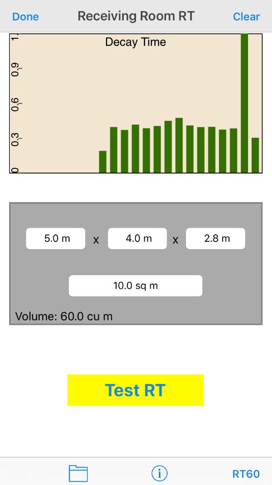
100 100 P a g e

101 Gated Noise RT P a g e

102 102 P a g e

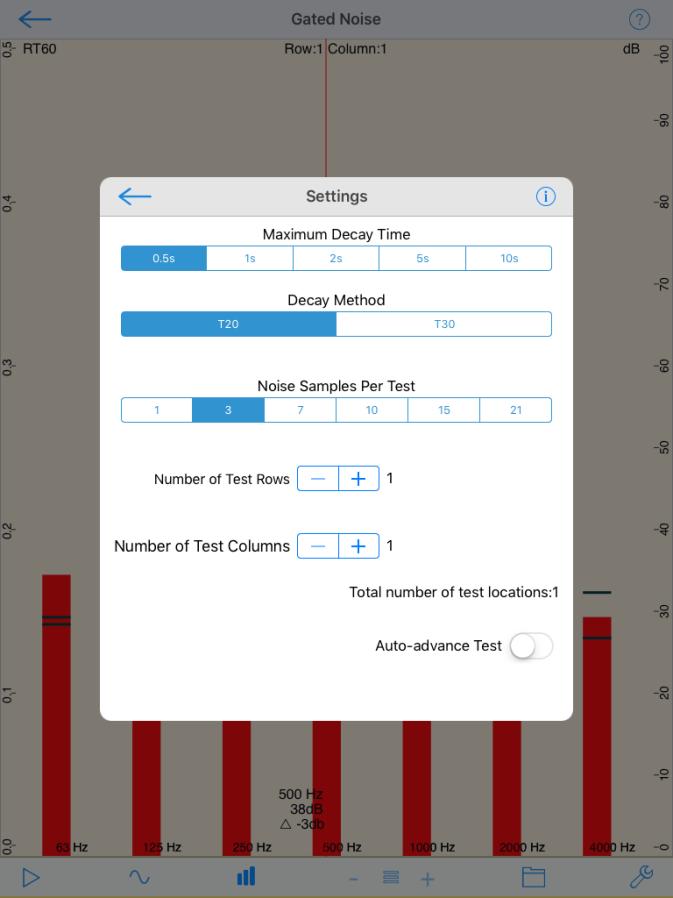
103 103 P a g e

104 LARSA LARSA is a powerful impulse response and analysis measurement tool. It is ideally suited for measuring loudspeakers in rooms, multi-speaker setups, car audio systems, home theatre systems or larger, installed speaker systems. The Basics LARSA is an acoustic measurement tool that mathematically compares a reference log sine chirp signal to that same signal measured through a transducer and room. This is useful, in that by subtracting the measured signal from the reference signal, what remains is just the impact of the speakers, other devices in the signal chain and any room interactions. There are a number of ways to record this signal. With our iaudiointerface2, you will plug in the line output of the interface into the input of the speaker you want to test. You will plug in your measurement microphone into the microphone input of the interface and set up the microphone in the location where you wish to measure the response. With our itestmic, the configuration will be the same, except you will use the line output of your ios device to feed the measurement signal into your system. Finally, you can use the internal microphone to capture the measurement signal, although for best results, a measurement microphone should be used. Setup The first step you need to perform is to take a reference measure to determine the latency of your system. Tap the wrench icon and in the ETC Graph setup screen you will see a Latency box. Set this to 0.0s that start. 104 P a g e

105 Then tap done place the microphone as close as you can to the transducer you wish to judge. Set the gain of your microphone preamp by tapping the Gear icon, and then Microphone Setup. For complete calibration and gain adjustment instructions, please refer to the instructions in the Settings screen. Tap the Measure button to take your first measurement, a log sine chirp signal will be recorded and through a process known as deconvolution, the resulting impulse will be generated. To set the latency, switch from the Analysis Curves screen to the ETC Screen by tapping the second grey icon on the bottom middle of the module. The ETC, or energy time curve shows how energy is decaying in your room. First, assure that the 1.00s option is selected in the ETC graph. Use a single finger drag to slide the cursor to the peak of the impulse response and observe the time readout. This is the reference latency of your system. Tap the wrench icon again, and type the time value you observe into the Latency field. This time tap the 0.020s button on the ETC Curve graph, your new measurement s peak should be 0 ms. If it is not, adjust your latency settings until your close mic is measuring 0 ms delay and distance. Once that is set, as you move around your room and make other measurement, the delays and distance differences will be meaningful. Basic Measurement There are two basic ways to use this module. The first is to make individual measurements of different loudspeakers or measurement locations around your room. The other is to make multiple spatially-averaged measurements of the same loudspeaker. We will start with the first case where you wish to measure a small studio monitor in a close microphone configuration (as close to the transducer as possible), at the listening location and then at multiple locations in the diffuse field. You have two options for chirp lengths, which can be selected in the setup screen. The 0.5s chirp give you good resolution and a quick measurement time. The 1.5s chirp gives you a bit more resolution in the lower frequencies, which is useful if you are measuring large loudspeakers that have an extended low frequency response or subwoofers. The chirp measures from 10 Hz - 22 khz, so please be careful of the output volume to your loudspeakers. Protect your hearing and your equipment. If you are measuring for an extended period of time, please use ear plugs. In the Audio section of the Setup pane, there is a Test Tone option, which will toggle a sine tone for level setting. Assure that the signal is intense enough, but not too loud that it will distort your microphone input. In addition to the chirp length setting, you can also select whether you are using a Balanced output or a Mono output, and select the input source. 105 P a g e

106 Back in the main screen, we are ready to make a measurement. Tap the 1 Test Number, position the microphone in the close microphone configuration (as close as you can get to the transducer). Now tap measure. In the Analysis Curves graph, you will see the frequency response of your measurement. The currently selected measurement in the Test Number will be traced in blue. Test Numbers that have a stored IR will be displayed in green text, and open locations will be displayed as red text. The Avg shows the average frequency response of all measurements. The frequency response graph can be smoothed. In the setup screen there are options for the Frequency Graph. Curve smoothing options from None to a full-octave smoothing are available. You can also manual set the ranges for the db (Y) axis, or frequency (X) axis. Next, move you microphone to the listening location (usually located in the sweet spot between your town monitor loudspeakers). Repeat the measurement process. Notice how the intensity of the frequency response has decreased because you are further away from the loudspeakers. Non of the responses are normalized in this module, so you can see the level differences and time difference in multiple measurements. Move over to the ETC Curves, assure that 0.020s is selected and notice how you can see that the second IR we ve measured is further back in time than the close mic IR. This is because there is a delay now introduced by the distance from the loudspeaker to the microphone. Drag your finger onto the plot the measure this delay. Line up the vertical cursor with the second peak and you will see the ms delay and the delay in distance. Move your microphone to the third measurement location and repeat the process. You can repeat this process for up to 8 measurement locations in the room.the store your results, tap the folder icon. For complete Save / Recall instructions, please refer to the info in this screen. If you have inadvertently made a spurious measurement, or wish to clear the memory in the Test Number boxes, highlight a Test, and tap the garbage icon. The module will prompt you the clear this test (the one highlighted), all tests or cancel. All tests will remove all of your measurements from memory, no matter which one is highlighted. Spatial Average Measurement A useful technique for characterizing how a loudspeaker sounds in a room is to measure a spatial average around the sweet spot. In the setup screen there is an option to show location prompts. Turning this on and selecting an analysis area similar to your listening configuration (single chair vs. a couch), will give you approximate locations for each of the 8 tests to measure. The technique here is to measure IRs around the listening location and take an average of all 8. This helps to smooth out modal behavior and gives you a reasonable impression of the frequency response that you are actually hearing. This technique is useful for setting tone controls, or equalization of your system. 106 P a g e

107 Start again by setting your latency as instructed above. Tap the test number 1 and place the microphone where the location prompt shows you to with the microphone pointing up at ear level. Continue the same process for the remains 7 measurements. Then tap the average button. This should be a reasonable approximation of the frequency response of your loudspeakers in your room. Note, you are not looking for a flat response here. Most systems that sound perceptually flat have a slight elevation of the response from 20 Hz - 20 Hz, are flat to 1 khz and then have a gradually dropping high frequency response towards 20 khz. To see just the Avg measurement, and not the individual ones, enter the setup screen and turn off the Show All Curve switch. Then tap done and tap the Avg Test Number. Measuring Multiple Speakers in the Same Location Another measurement technique that you can use Room EQ for is to make measurements of multiple loudspeakers at the same location. We will take the case of measuring a 5.1 surround sound system in the sweet spot of a home theatre. Again, start by making the reference latency measurement, and then place the microphone in the sweet spot with the diaphragm pointing up. Tap test number 1, and route the signal to the left loudspeaker. Measure the response. Tap test number 2, route the signal to the centre signal and measure the response. Continue measuring the right, right surround, left surround and subwoofer in the same way. Now you can compare the frequency response of each loudspeaker as well as the arrival time by inspecting the ETC Curves Screen. Video The video for Larsa is on Youtube: P a g e

108 Transfer Function The Studio Six Digital Transfer function includes the most-used Transfer Function features in an easyto-use GUI package. With Transfer Function, you can make changes to a sound system without having to run pink noise or swept sine waves through the system. This allows you to monitor system performance, or make adjustments, while the system is in use and the crowd is in the room. See the demo video of Transfer Function: The User manual is found at: Transfer Function is by definition a dual-channel measurement, and so to use it you need to either use a two-channel input device, or you will use the signal generator as the reference signal. iaudiointerface2 was designed specifically with Transfer Function in mind, since it includes a microphone input, and a second line input for the reference signal. You can also use other two-channel interfaces, such as the original iaudiointerface or many of the generic 2-channel audio interfaces that work with ios. Using Transfer Function With A SIngle-Channel Input Device Transfer Function can be used with a single-channel input device, such as the built-in ios device microphone, itestmic, or iprecisionmic. In this case, you have to use the signal generator to make the reference signal. To do this, you will need to use a cable that has an 1/8" TRS 3-conductor plug on the end that plugs into the ios device. If the plug has 4 conductors, the ios device will turn off the built-in mic and look 108 P a g e

109 for a mic on that cable. The other end of the cable might be 2 RCA connectors, or it could be wired to an XLR or 1/4" TRS plug. If you are using 2 RCA connectors, make sure you select "mono" for the generator output. If you are wiring to a balanced connector, like an XLR or 1/4" TRS, make sure you select "balanced" for the generator output. Selecting the wrong mode will result in attenuated low frequency readings. Next, make sure that the output cable is the last thing that you plug into the ios device. Plug in the itestmic or iprecisionmic first, and then plug in the output cable. Now open the generator panel by tapping the sine wave icon, select pink noise, and turn the generator on. Next, start the Transfer Function running, using the Play/Pause button on the toolbar. You should start to get results at this time. Continue to the other steps described below, including setting the delay, to get accurate results. Transfer Function on ipad Here is Transfer Function on ipad, showing a running trace (green and blue), and a recalled trace (yellow and magenta). The coherence plots for both measurements are shown, in red and dark red: Included in Transfer Function are: 109 P a g e

110 Magnitude Graph The magnitude graph is used to show the difference between the reference signal and the test signal. Typically, the reference signal is pink noise, although you can also use mono program material (music) and still get good results. The graph auto-centers around the 0 db axis, so it's easy to see how the test signal differs from the reference signal. Phase Graph The phase graph shows the relative phase of the signal, and is useful for setting crossover points. Coherence Graph The coherence graph is used as a measure of the reliability of a set of averaged transfer function measurements. 100% would mean that you are seeing highly correlated graphs, and thus the information on the magnitude and phase graphs would be accurate. Coherence Blanking It may be useful to only display transfer function plot data when the coherence is above a certain threshold. This helps you know that the information being shown is reliable. To do this, you can set a coherence blanking threshold in percent, on the setup screen. When the blanking threshold is greater than 0, plot data will only be shown that has a corresponding coherence greater than the threshold. Typical coherence blanking values are 20-50%. Delay Finder Transfer Function includes a sample-accurate, impulse-response based delay finder. This is a very powerful feature, and is used to set the delay for the most accurate Transfer Function measurements, and it can also be used as a standalone delay finder, to accurately measure the time arrival of a signal, for setting driver delays times. Using Delay Finder to Set Up Transfer Function Since it is critical that the time offset between the reference and test signal is known, there has to be a way to accurately compute the time delay between these signals. Our impulse response based delay finder does just this. Just tap the delay value to bring up the Delay Finder panel. Select an FFT size, which sets the longest delay that you can measure, and tap Find. The delay will be computed, and shown on the screen. To average more than one FFT, enter a number larger than 1 in the Averages field. Averaging several FFTs can increase the accuracy of the results. 110 P a g e

111 To calibrate the system to run the Transfer Function, place the microphone at the location that you will be testing, run the delay finder, and tap Set as Baseline. This is important, because the phase plot will not be correct if you have not time-aligned the output to the input. Using Delay Finder to Time-Align Loudspeakers To calibrate the system to compute relative delays, place the microphone at your zero distance. This may be the speaker grill, or the plane of the front of the driver that you are testing. Run the Delay Finder, and tap Set as Baseline. Now, you can move the microphone to a different location, run the delay finder again, and see the exact delay in time and distance. You can also enter the temperature of the air in the room, to get the most accurate distance calculations. You can also change to another driver, and compare the delay for this driver to your reference driver. If you get negative delays, that means that the driver you are testing has less delay than the one you used to set the baseline. Just reset the baseline to zero out this driver, and go back to the other one and remeasure it. Note on Using The Internal Generator When you are using the internal generator, the first time that compute the delay you may notice a very large delay time and distance being computed. This is normal when using the internal generator, and the built-in mic or an external microphone. It is due to the iphone audio latency between the ios audio output and input that varies greatly, from device to device, and even from one run to the next. Follow the instructions above to correct this delay. Setup 111 P a g e

112 Select the FFT size and windowing, display type, turn Peak Tracking on or off. Select the SPL readout and decay speed. The Measure Source and Reference Source are selected from this screen. The Coherence Blanking percent will blank out parts of the magnitude and phase plot that have coherence lower than the value. The switch turns the Coherence plot on or off. You can also engage Difference Plot Mode, control audio pass-through, turn on Difference mode. The graph scales may be set manually, and you can lock the graph scale so that the touch-gui is disabled. The Phase plot may be smoothed, or you can leave it unsmoothed to see the full phase detail. You can also select whether or not you want to wrap the phase plot when it exceeds the plot bounds. Using Transfer Function with itunes When you are using iaudiointerface2, it's easy to use music as the test signal source for Transfer function. To do this, you will have to run at 44.1kHz sample rate, because itunes will not run at 48kHz, which is the sample rate that we 112 P a g e

113 STIPA PRO STIPA is the most advanced speech intelligibility process available. It is rapidly being accepted by and required by fire codes in the United States and other countries. The determination of the Speech Transmission Index (STI) was developed in order to quantify the reduction of the modulation envelope of speech by means of calculating the modulation transfer function (MTF) (Steeneken and Houtgast, 1980). The STI measure has been defined in IEC :2011, and provides an efficient method of evaluating speech intelligibility in both unamplified direct conversations as well as when the speaker is amplified through a public address (PA) system. This is due to the fact that the STI takes into account distortions due to noise, reverberation and echoes, if present. With STIPA Pro, you get both the single-number value as required by codes, and the octave-band values. You can also view all of the detail on another screen, save and recall results, and detailed results from the app. Or, for a more affordable STIPA measurement that still meets all of the requirements of the specification, download our STIPA Basic module. Purchasers of STIPA Pro also automatically get access to STIPA Basic. The test signal is supplied, and is available for download from this web site. You can burn it to a CD, or copy it to any audio player. When you first access a STIPA test signal from the app, the audio file will be downloaded. Or, you install them all directly using itunes. The Studio Six version is fully compliant with v4 of the standard (IEC :2011). Download the Studio Six STIPA Compliance Study, which documents how the STIPA module meets IEC :2011. This document is also available from the Acoustar library, Module 5, Instrumentation. 113 P a g e

114 ACU AUDIO COVERAGE UNIFORMITY One of the fundamental goals of sound system performance for both speech reinforcement and program audio is the delivery of consistent coverage in the listening area. A well-executed audio system design is one that allows all listeners to hear the system at approximately the same sound pressure level throughout the desired frequency spectrum range, no matter where positioned in the designated listening area. 114 P a g e

115 115 P a g e

116 TECHNICAL APP NOTES db vs. db Understanding SPL Measurements AudioTools provides many options for measuring and analyzing sound. A number of these include SPL db values, and although they may all be displayed as a single numeric value, they may mean different things, or have different values. We will try to explain these differences here. Overall SPL db The most common measure is a simple overall, or wide-band, SPL db value. This appears in many locations: SPL Meter SPL Pro SPL Traffic Light RTA graph, upper right corner FFT graph, upper right corner Smaart Tools, upper left corner Microphone Calibration, db field This value is dynamic representation of the overall sound level in the room. It will vary as the sound in the room is louder or softer -- unless, that is, you are in Leq mode. Leq simply means sound energy average over time. So an Leq10 will typically be the average SPL level over 10 minutes. The overall SPL level usually has a weighting applied to it. A weighting is simply a filter, or set of filters, that alter the effect of certain frequencies on the reading. Common weightings are A and C. Note in the graph below that A weighting removes a lot of energy in the low frequencies, as well as attenuating high frequencies, while C removes much less of the lows, and still some highs. Some people think of A-weighting as "voice" and C-weighting as "music". 116 P a g e

117 Given the difference between A-weighting and no weighting, if the ambient sound in the room has a lot of low frequencies (which are less audible, see curve below), then the difference between a A- weighted SPL reading and an unweighted SPL reading could be db or more. Here's how this works in AudioTools. Say you open SPL Meter, which has only A and C weighting, and leave it set to A. The reading might be 35dB, in a typical quiet room. Now switch to RTA (which has choices for overall weighting, A, C, or none) or FFT (which only supports choices for weighting on some platforms and otherwise is "none"), and you might see 55dB. Which number is right? Both, of cthese, but they will not match unless the same weighting is selected for both measures. Octave or Fractional Octave Band db Now we will look at how breaking up the audio spectrum into bands effects the db levels that are displayed. Say we have pink noise (which is wide-band noise filtered so that each octave or fractional octave band has the same energy, the same way that the ear hears it) at 80dB. What will the RTA show for the level of each octave band? The answer is not 80 db. A good way to visualize this is to remember that 80 db really refers to an amount of acoustic energy. If we break up the audio spectrum into 10 bands, each band would hold 1/10 the energy of the total. But to add them, since we are working in db, it is not a linear formula -- otherwise each band would be 8 db! The formula for the increase in summing equal loudness sources is db = 10 * log10( n ) db to add for n sources Where n is the number of sources. For n = 10, the answer is 10. So, if the overall level was 80 db, each octave band would be 70 db. If you switch to 1/3 octave, the amount to add is 14.7 db, so each band would be 65.3 db. What about sine waves? In this case, if we have a sine wave at 75 db at 1000Hz, the 1000Hz octave or 1/3 octave band will read 75 db, and the overall will show something slightly higher than 75 db, since it adds the single band energy (75) with the other bands, again using a log10 formula. Equal Loudness Curves and Threshold of Hearing Here is graph that shows how the human ear perceives loudness, by frequency and SPL level. The thing that is really obvious is at quiet levels, we don't really hear low frequencies. In fact, we can't even hear 60Hz until it's above 40dB, and we can't hear 20Hz until it reaches over 70dB! 117 P a g e

118 So this is why an unweighted SPL reading might show 50 or 60 db, in what we consider a very quiet room. The RTA or FFT will show the actual sound levels, and so become very useful tools for understanding the entire sound spectrum in a room. 118 P a g e

119 Headset Connected Microphones The headset mic input on all current ios devices uses the same filter as the built-in mic, (depending on ios version) and so offers no improvement to performance over the built-in mic. Because of this, we can't recommend any mic that plugs into the headset connector, such as micw. Although micw may perhaps be using a higher quality capsule than the iphone mic capsule, since it is using the headset mic input, it is subject to the same filters and Apple analog electronics as the built-in mic. Again, even in ios 6, we see no improvement in frequency response, or flatness over the Apple built-in mic, with micw. micw does have lower sensitivity, so it will clip at a higher SPL point, although it's noise floor is also therefore higher, so it can't measure as low of noise levels. The calibration we normally see for this mic is around +13. Connecting an External Mic The headphone / input jack on ios devices has a 4th pin that has a small polarizing voltage on it with very low drive current. The Apple device monitors this line, and can tell when a typically headset mic is plugged in. If its not, they don't even turn on the mic input. Most people don't have very much success connecting a non-apple mic to this port. Some of the third-party mics, like MicW and IMM6, do use this input, but really they are just swapping one small mic capsule for another. No great improvement here. Also, there are no analog inputs on either the 30-pin or Lightning jack, so its not possible to connect something there. Really the only way to get an external mic into an ios device is with one of the third-party adapters, like for example the iaudiointerface2 or itestmic, which convert the mic signal to digital audio before routing it to the ios device. Another Flaw in the Headset Jack We have recently discovered another major flaw in the Apple headset connector. It seems that the way that Apple has implemented the headset jack as an input and output connector, when the output is active, it bleeds back into the mic input. This bleed can easily overpower the mic input signal, rendering the input completely useless. The bleed gets worse as the output load impedance goes down, and as the output level increases. Using a typical high-impedance input, such as the line input on a consumer receiver, the bleed may be low enough that if the acoustic level in the room is fairly high, it won t make much of a difference to the measurement. The bleed is much worse when the generator is in mono mode, since the left 119 P a g e

120 and right channels are both sending out the same signal. In balanced mode, the problem nearly disappears. However, in balanced mode, the signal to each channel gets distorted, apparently due to the crosstalk between the channels. The summary is that if you do plug a mic into the headset jack, don t use the output. Even turning on the output with no load attached can cause phantom readings rising up to +20 db at 20 khz. The amount of this bleed, or crosstalk, varies widely from model to model. In every case, there is at least 20 db of boost at 20kHz. In some devices there is as much as 50 db wide band across the entire audio spectrum. Audio Output You can get audio out of most ios devices just by making a cable and plugging it into the ios device headset jack. The first trick is that the cable has to be an 1/8" 3-conductor plug. If it is a 4-conductor plug, the ios device will switch its input to the headset jack, since it is sensing a microphone being plugged in. You can make a number of different cables, including a stereo output cable, for example to have right and left RCA plugs, and you can also make a balanced cable, by connecting the tip of the 1/8" plug to the balanced +, and the ring to the balanced connector -. Just make sure you set the generator in AudioTools to match the type of cable you are using. The second trick is that you have to plug this cable into the headset jack after connecting itestmic. ios has a rule that "the last one connected wins", so you have to plug this in last to grab the output audio away from the digital audio going to itestmic. 120 P a g e

121 itestmic Information Applications itestmic works with all of the acoustic testing modules in AudioTools, including the SPL Meters, RTA, FFT, ETC, Impulse Response, and now with Transfer Function, using the internal signal generator. Specifications Omnidirectional pattern 20Hz - 20kHz +/- 3dB 28 dba dba performance in two ranges NC Limit: Below NC29 1/2" nominal size, fits all standard calibrators Consumes less than 50ma in use 0.5m (19") cable length (30-pin) 1.0m (37 ) cable length (Lightning) Two gain ranges, dba, and dba Mono signal, present at both Left and Right ios device input channels Excellent immunity to cell phone RF noise Factory calibration stored internally, from a 94.0 db pressure-compensated calibrator. Technical Information Every itestmic2 microphone is calibrated during production at our US facility for SPL level using a state-of-the art pressure-compensated Class 1 microphone calibrator. The Low and High range trim factors are stored in the microphone's non-volatile memory, and so when itestmic2 is plugged into an ios device running one of our apps, the calibration is automatically read and applied to calibrate the level and provide accurate SPL readings with no calibration required. All microphones deviate from flat frequency response, and to optimize the frequency readings from itestmic2, we first test every unit to be within tight standards of frequency response, and then we 121 P a g e

122 go one more step. Using a Class 1 iprecisionmic as the standard, we create an individual frequency compensation file for each microphone. The files are stored in the Amazon cloud by unique serial number, and can be installed in any Studio Six Digital app with a single button tap. To install the frequency calibration file, plug itestmic2 into your ios device running any of our apps, including AudioTools, and navigate to the Microphone Calibration page. Tap the "Get File" button, and the file is located using the unique serial number in itestmic2, downloaded, and automatically applied. Once downloaded, the file will then be applied each time the itestmic2 is plugged in. The frequency calibration files are stored permanently on our servers hosted by Amazon, and will be available to download anytime you install our apps on a new ios device. This is a typical curve, after the frequency calibration file has been applied. The LF bumps are artifacts from the pink noise cycling. Getting the Generator Output Signal Some AudioTools modules require an output signal from the ios device. It s easy to get this signal on most ios devices. First, make or obtain a cable with a 3-conductor 1/8 TRS (not the 4-conductor plug, which is meant for microphone access). Set up the generator in AudioTools for balanced or mono mode, depending on the other end of the cable. If you are going 1/8 to XLR or 1/4 TRS, selected Balanced. If you are going to dual RCA plugs, select MONO. Then, after you have plugged itestmic into the ios device, plug the 1/8 TRS cable into the headset jack. ios will now route the output signal automatically to the headset jack. 122 P a g e

123 iprecisionmic Sound Analysis System iprecisionmic is a precision, professional microphone that is also an ios direct-connect Lightning accessory. iprecisionmic is factory calibrated to +/-0.1dB using a NIST traceable pressurecompensated calibrator. The calibration offsets are store in the microphone s non-volatile memory, and are transferred automatically to an ios device running the AudioTools app. All of the active electronics are in the microphone body, including the regulated power supply, microphone preamplifier, precision 24-bit A/D converter, and the circuitry required to communicate with Apple devices via a digital audio link. This means that we are not reliant on the analog electronics stages in the iphone or ipad, but rather we completely bypass them with a digital audio link. Features Meets Class 1 acoustical specifications for sound level meter per ANSI S and IEC :2002 and 60804:2000 Type 1. Meets Class 1 for ANSI S1.11 / IEC 61260:1995 Class 0 Octave and Fractional Octave Band Digital Filters, frequency range from 32Hz to 16kHz in octave bands, and 25Hz to 20kHz in 1/3 octave bands. Certification available. Fast, Slow, Impulse, Max, Min, Leq, Ln. Octave and 1/3 Octave logging. Z-, A-, or C-weighted spectra. Connect iprecisionmic to any ios device with a Lightning connector, download the AudioTools app, and you have a precision sound level meter, ready for certification. Plug in the included AC adapter and charge the attached ios device for extended run time. 123 P a g e

124 iprecisionmic Calibration certificate Instruments: iphone 6, iprecision preamplifier, ACO Class 1 microphone, AudioTools RTA and SPL Pro apps 124 P a g e

125 125 P a g e

126 126 P a g e

127 iaudiointerface2 iaudiointerface2 and included ios Lightning and USB Audio interconnect cables. The professional audio interface for ios devices made to work with for AudioTools. Phantom powered mic input, balanced line input and output, digital audio output, internal battery, and ios device charging. Technical Information All specifications subject to change. Please read the User manual with the interface module. Microphone Input Standard XLR microphone connector. Switchable 48V phantom power available that meets all specs for voltage and current. Input gain 0dB to +50dB in 9 preset gain stages, set from within AudioTools. Equivalent Input Noise gain -112dBu A-weighted. Microphone appears to ios app as left input channel. Input impedance 20k Ohms. Input THD < 0.005% at 1kHz, -1dBFS, battery powered. Frequency response -0.3/ kHz. Digital Audio Output Optical Toslink PCM digital audio output, sample rate 32k/44.1k/48k, set from ios device. 16-bit (current ios maximum). Supports output of Dolby Digital AC3 Dolby Digital 5.1 test signals, and DTS- ES 6.1 test signals, optional in AudioTools. Requires ios5. Line Input Fully balanced 1/4" TRS line input, appears to ios app as the right input channel. May be switched to a stereo unbalanced input. Input Impedance 40k Ohms balanced, 20k Ohms unbalanced. THD < kHz, -1dBFS, battery powered. 127 P a g e

128 Three gain ranges, selected from AudioTools: -80dBU to -10dBu -60dBu to +15dBu -40dBu to +40dBu Line Output Fully balanced 1/4" TRS mono line output. Maximum output level +12dBu THD < -1dBFS, battery powered. Output may be switched to stereo, suitable to drive 32 Ohm headphones. ADC and D/A Converters For dock-connector digital audio, the ios device sets the sample rate and bit depth of the signal. Currently Apple supports 32kHz, 44.1kHz, and 48kHz sample rates, all at a bit depth of 16 bits. We license a proprietary high-resolution USB clock recovery algorithm that provides a highly stable timebase for our converters. This recovered-clock digital audio signal is presented unaltered at the optical TosLink output. Sample rate converters are never used in our hardware. iai2 uses Wolfson stereo codec with a 24-bit multi-bit sigma delta ADC and switched capacitor multibit sigma delta DACs, which operates at an oversampling rate of 128fs for both ADC and DAC. Internal li-ion Battery Charge time 2-3 hours. Run time 3-5 hours depending on usage. To prevent running down the battery when iaudiointerface2 is not being used, always unplug it from the ios device when you are not using it. Even though most circuits are shut off when audio is not running, it will still consume the battery once it has been connected and identified by the ios device. When battery is being charged, and an ios device is attached, the charge LED will light. ios Device Charging High-current charging is designed for ipad, and will also fast-charge iphone 4 and ipod touch 4. Charging occurs anytime that the AC adapter is plugged. Charger Specifications Includes universal 100VAC - 230VAC charger 50/60Hz, with 4 common prong adapters: US, EU, UK, and Australian. iaudiointerface2 requires 5V DC at 4Amp, 5.5mm connector with 2.1mm pin, pin positive. 128 P a g e