Operator's Manual WaveSurfer 510 Oscilloscopes

Transcription

1 Operator's Manual WaveSurfer 510 Oscilloscopes

2 WaveSurfer 510 Oscilloscope Operator's Manual 2017 Teledyne LeCroy, Inc. All rights reserved. Unauthorized duplication of Teledyne LeCroy, Inc. documentation materials other than for internal sales and distribution purposes is strictly prohibited. However, clients are encouraged to duplicate and distribute Teledyne LeCroy, Inc. documentation for their own internal educational purposes. WaveSurfer and Teledyne LeCroy, Inc. are trademarks of Teledyne LeCroy, Inc., Inc. Other product or brand names are trademarks or requested trademarks of their respective holders. Information in this publication supersedes all earlier versions. Specifications are subject to change without notice Rev B May 2017

3 Contents Safety 1 Symbols 1 Precautions 1 Operating Environment 2 Cooling 2 Cleaning 2 Power 3 Oscilloscope Overview 5 Front of Oscilloscope 5 Side of Oscilloscope 6 Back of Oscilloscope 7 Front Panel 8 Signal Interfaces 11 Oscilloscope Set Up 13 Powering On/Off 13 Software Activation 13 Connecting to Other Devices/Systems 14 Language Selection 15 Using MAUI 17 Touch Screen 17 OneTouch Help 24 Working With Traces 31 Zooming 34 Print/Screen Capture 36 Acquisition 37 Auto Setup 37 Viewing Status 38 Vertical 38 Digital (Mixed Signal) 42 Timebase 45 Trigger 52 Display 63 Display Set Up 64 Persistence Display 66 i

4 WaveSurfer 510 Oscilloscope Operator's Manual Math and Measure 69 Cursors 69 Measure 72 Math 79 Memory 91 Analysis Tools 93 WaveScan 93 Pass/Fail Testing 97 Saving Data (File Functions) 99 Save 99 Auto Save 104 Recall 105 LabNotebook 107 Report Generator 112 Share 113 Print 114 & Report Settings 115 Using the File Browser 116 Utilities 119 Utilities Dialog 119 Status 119 Remote Control 120 Auxiliary Output 122 Date/Time 123 Options 124 Disk Utilities 125 Preferences Settings 126 Calibration 127 Acquisition 129 Miscellaneous 130 Maintenance 131 Touch Screen Calibration 131 Reboot Instrument 131 Firmware Update 132 Technical Support 133 Returning a Product for Service 134 ii

5 Certifications 135 EMC Compliance 135 Safety Compliance 136 Environmental Compliance 137 ISO Certification 137 Warranty 138 Intellectual Property 138 Windows License Agreement 138 Index 139 iii

6 WaveSurfer 510 Oscilloscope Operator's Manual Welcome Thank you for purchasing a Teledyne LeCroy WaveSurfer oscilloscope. We're certain you'll be pleased with the detailed features unique to our instruments. Take a moment to verify that all items on the packing list or invoice copy have been shipped to you. Contact your nearest Teledyne LeCroy customer service center or national distributor if anything is missing or damaged. We can only be responsible for replacement if you contact us immediately. We truly hope you enjoy using Teledyne LeCroy's fine products. Sincerely, David C. Graef Vice President and General Manager, Oscilloscopes Teledyne LeCroy iv

7 Safety Safety To maintain the instrument in a correct and safe condition, observe generally accepted safety procedures in addition to the precautions specified in this section. The overall safety of any system incorporating this product is the responsibility of the assembler of the system. Symbols These symbols appear on the instrument or in documentation to alert you to important safety concerns: Caution of potential damage to instrument or Warning of potential bodily injury. Do not proceed until the information is fully understood and conditions are met. Caution, high voltage; risk of electric shock or burn. Caution, contains parts/assemblies susceptible to damage by Electrostatic Discharge (ESD). Frame or chassis terminal (ground connection). Alternating current. Standby power (front of instrument). Precautions Caution: Comply with the following to avoid personal injury or damage to your equipment. Use indoors only within the operational environment listed. Do not use in wet or explosive atmospheres. Maintain ground. This product is grounded through the power cord grounding conductor. To avoid electric shock, connect only to a grounded mating outlet. Connect and disconnect properly. Do not connect/disconnect probes, test leads, or cables while they are connected to a live voltage source. Observe all terminal ratings. Do not apply a voltage to any input that exceeds the maximum rating of that input. Refer to the body of the instrument for maximum input ratings. Use only power cord shipped with this instrument and certified for the country of use. Keep product surfaces clean and dry. See Cleaning. Do not remove the covers or inside parts. Refer all maintenance to qualified service personnel. Execise care when lifting. Use the built-in carrying handle. Do not operate with suspected failures. Do not use the product if any part is damaged. Obviously incorrect measurement behaviors (such as failure to calibrate) might indicate hazardous live electrical quantities. Cease operation immediately and secure the instrument from inadvertent use. 1

8 WaveSurfer 510 Oscilloscope Operator's Manual Operating Environment Temperature: 5 to 40 C. Humidity: Maximum relative humidity 80 % for temperatures up to 31 C, decreasing linearly to 50% relative humidity at 40 C. Altitude: Up to 3,000 m at or below 25 C. Cooling The instrument relies on forced air cooling with internal fans and vents. Take care to avoid restricting the airflow to any part. In a benchtop configuration, leave a minimum of 15 cm (6 inches) around the sides between the instrument and the nearest object. The feet provide adequate bottom clearance. Follow rackmount instructions for proper rack spacing. Caution: Do not block the cooling vents. The instrument also has internal fan control circuitry that regulates the fan speed based on the ambient temperature. This is performed automatically after start-up. Cleaning Clean only the exterior of the instrument using a soft cloth moistened with water or an isopropyl alcohol solution. Do not use harsh chemicals or abrasive elements. Under no circumstances submerge the instrument or allow moisture to penetrate it. Dry the instrument thoroughly before connecting a live voltage source. Caution: Unplug the power cord from the AC inlet before cleaning to avoid electric shock. Do not attempt to clean internal parts. Refer all maintenance to qualified service personnel. 2

9 Safety Power AC Power The instrument operates from a single-phase, Vrms (± 10%) AC power source at 50/60 Hz (± 5%) or a Vrms (± 10%) AC power source at 400 Hz (± 5%). Manual voltage selection is not required because the instrument automatically adapts to the line voltage. Power Consumption Maximum power consumption with all accessories installed (e.g., active probes, USB peripherals) is 375 W (375 VA). Power consumption in Standby mode is 15 W. Ground The AC inlet ground is connected directly to the frame of the instrument. For adequate protection again electric shock, connect to a mating outlet with a safety ground contact. Caution: Use only the power cord provided with your instrument. Interrupting the protective conductor (inside or outside the case), or disconnecting the safety ground terminal, creates a hazardous situation. Intentional interruption is prohibited. 3

10 WaveSurfer 510 Oscilloscope Operator's Manual 4

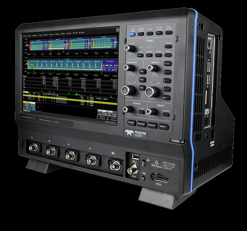
11 Oscilloscope Overview Oscilloscope Overview Front of Oscilloscope A. Touch screen display G. Aux output B. Front panel H. USB port C. Stylus holder D. Power button E. Channel inputs (C1-C4) F. Ext input I. Ground and Calibration output terminals J. LBUS input K. Tilting feet 5

12 WaveSurfer 510 Oscilloscope Operator's Manual Side of Oscilloscope A. HDMI port for external monitor B. DisplayPort port for external monitor C. USB 3.1 ports (4) D. Ethernet ports (2) for connecting to LAN or remote control E. Audio In/Out (mic and speaker ) for connecting external audio devices 6

13 Oscilloscope Overview Back of Oscilloscope A. Built-in carrying handle B. AC power inlet C. Kensington lock 7

14 WaveSurfer 510 Oscilloscope Operator's Manual Front Panel Front panel controls duplicate functionality available through the touch screen and are described here only briefly. Knobs on the front panel function one way if turned and another if pushed like a button. The first label describes the knob s turn action, the second label its push action. Actions performed from the front panel always apply to the active trace. Many buttons light to show the active traces and functions. Trigger Controls Level knob changes the trigger threshold level (V). The level is shown on the Trigger descriptor box. Pushing the knob sets the trigger level to the 50% point of the input signal. READY indicator lights when the trigger is armed. TRIG'D indicator is lit momentarily when a trigger occurs. Setup opens/closes the Trigger Setup dialog. Auto sweeps after a preset time, even if the trigger conditions are not met. Normal sweeps each time the trigger signal meets the trigger conditions. Single sets Single trigger mode. The first press readies the oscilloscope to trigger. The second press arms and triggers the oscilloscope once (single-shot acquisition) when the input signal meets the trigger conditions. Stop pauses acquisition. If you boot up the instrument with the trigger in Stop mode, a "No trace available" message is shown. Press the Auto button to display a trace. Horizontal Controls The Delay knob changes the Trigger Delay value (S) when turned. Push the knob to return Delay to zero. The Horizontal Adjust knob sets the Time/division (S) of the acquisition system when the trace source is an input channel. The Time/div value is shown on the Timebase descriptor box. When using this control, the instrument allocates memory as needed to maintain the highest sample rate possible for the timebase setting. When the trace is a zoom, memory or math function, turn the knob to change the horizontal scale of the trace, effectively "zooming" in or out. By default, values adjust in 1, 2, 5 step increments. Push the knob to change to fine increments; push it again to return to stepped increments. 8

15 Vertical Controls Oscilloscope Overview Offset knob adjusts the zero level of the trace (making it appear to move up/down relative to the center axis). The voltage value appears on the trace descriptor box. Push the knob to return Offset to zero. Gain knob sets vertical scale (V/div). The voltage value appears on the trace descriptor box. By default, values adjust in 1, 2, 5 step increments. Push the knob to change to fine increments; push it again to return to stepped increments. Channel (number) buttons turn on a channel that is off, or activate a channel that is already on. When the channel is active, pushing its channel button turns it off. A lit button shows the active channel. Dig button enables digital input through the Digital Leadset on instruments with the Mixed Signal option. Math, Zoom, and Mem(ory) Buttons The Zoom button creates a quick zoom for each open channel trace. Touch the zoom trace descriptor box to display the zoom controls. The Math and Mem(ory) buttons open the corresponding setup dialogs. If a Zoom, Math or Memory trace is active, the button illuminates to indicate that the Vertical and Horizontal knobs will now control that trace. Cursor Controls Cursors identify specific voltage and time values on a waveform. The white cursor markers help make these points more visible. A readout of the values appears on the trace descriptor box. There are five preset cursor types, each with a unique appearance on the display. These are described in more detail in the Cursors section. Type selects the cursor type. Continue pressing to cycle through all cursor until the desired type is found. The type "Off" turns off the cursor display. Cursor knob repositions the selected cursor when turned. Push it to select a different cursor to adjust. Adjust and Intensity Controls The front panel Adjust knob changes the value in active (highlighted) data entry fields that do not have dedicated knobs. Pushing the Adjust knob toggles between coarse (large increment) or fine (small increment) adjustments. When more data is available than can actually be displayed, the Intensity button helps to visualize significant events by applying an algorithm that dims less frequently occurring samples. This feature can also be accessed from the Display Setup dialog. 9

16 WaveSurfer 510 Oscilloscope Operator's Manual Miscellaneous Controls Auto Setup performs an Auto Setup. Default Setup restores the factory default configuration. Print captures the entire screen and outputs it according to your Print settings. It can also be configured to output a LabNotebook entry. Touch Screen enables/disables touch screen functionalilty. Clear Sweeps resets the acquisition counter and any cumulative measurements. Decode opens the Serial Decode dialog if you have serial data decoder options installed. WaveScan opens the WaveScan dialog. Spectrum opens the Spectrum Analyzer dialog if you have that option installed. History opens the History Mode dialog. 10

17 Signal Interfaces Oscilloscope Overview The instrument offers a variety of interfaces for using probes or other devices to input analog or digital signals. See the product page at teledynelecroy.com for a list of compatible devices. Analog Inputs A series of connectors arranged on the front of the are used to input analog signals on channels 1-4. WaveSurfer 510 channel connectors use the ProBus interface. The ProBus interface contains a 6-pin power and communication connection and a BNC signal connection to the probe. It includes sense rings for detecting passive probes and accepts a BNC cable connected directly to it. ProBus offers 50 Ω and 1 MΩ input impedance and control for a wide range of probes. The channel interfaces power probes and completely integrate the probe with the channel. Upon connection, the probe type is recognized and some setup information, such as input coupling and attenuation, is performed automatically. This information is displayed on the Probe Dialog, behind the Channel (Cx) dialog. System (probe plus instrument) gain settings are automatically calculated and displayed based on the probe attenuation. Probes The oscilloscope is compatible with the included passive probes and most Teledyne LeCroy active probes that are rated for the instrument s bandwidth. Probe specifications and documentation are available at teledynelecroy.com/probes. Passive Probes The passive probes supplied are matched to the input impedance of the instrument but may need further compensation. Follow the directions in the probe instruction manual to compensate the frequency response of the probes. Active Probes Most active probes match probe to oscilloscope response automatically using probe response data stored in an on-board EEPROM. This ensures the best possible combined probe plus oscilloscope channel frequency response without the need to perform any de-embedding procedure. Be aware that many active probes require a minimum oscilloscope firmware version to be fully operational. See the probe documentation. LBUS Interface The LBUS (LeCroy Peripheral Bus) interface provides precise timing synchronization between the oscilloscope and external devices. 11

18 WaveSurfer 510 Oscilloscope Operator's Manual 12

19 Oscilloscope Set Up Oscilloscope Set Up Powering On/Off Press the Power button to turn on the instrument. The X-Stream application loads automatically when you use the Power button. Caution: Do not change the instrument s Windows Power Options setting from the default Never to System Standby or System Hibernate. Doing so can cause the system to fail. Caution: Do not power on or calibrate with a signal attached. The safest way to power down the oscilloscope is to use the File > Shutdown menu option, which will always execute a proper shut down process and preserve settings. Quickly pressing the power button should also execute a proper shut down, but holding the Power button will execute a hard shut down (as on a computer), which we do not recommend doing because it does not allow the Windows operating system to close properly, and setup data may be lost. Never power off by pulling the power cord from the socket or powering off a connected power strip or battery without first shutting down properly. The Power button does not disconnect the instrument from the AC power supply. The only way to fully power down the instrument is to unplug the AC power cord. We recommend unplugging the instrument if it will remain unused for a long period of time. Software Activation The operating software (firmware and standard applications) is active upon delivery. At power-up, the instrument loads the software automatically. Firmware Free firmware updates are available periodically from the Teledyne LeCroy website at: teledynelecroy.com/support/softwaredownload Registered users can receive an notification when a new update is released. Follow the instructions on the website to download and install the software. Purchased Options If you decide to purchase an option, you will receive a license key via that activates the optional features. See Options for instructions on activating optional software packages. 13

20 WaveSurfer 510 Oscilloscope Operator's Manual Connecting to Other Devices/Systems Make all desired cable connections. After start up, configure the connections using the menu options listed below. More detailed instructions are provided later in this manual. LAN The instrument accepts DHCP network addressing. Connect a cable from the Ethernet port on the side panel to a network access device. Go to Utilities > Utilities Setup > Remote to find the IP address. To assign a static IP address, choose Net Connections from the Remote dialog. Use the standard Windows networking dialogs to configure the device address. Choose File > File Sharing and open the & Report Settings dialog to configure settings. USB Peripherals Connect the device to a USB port on the front or side of the instrument. These connections are "plug-andplay" and do not require any additional configuration. Printer WaveSurfer 510 oscilloscopes support USB printers compatible with the instrument's Windows OS. Go to File > Print Setup and select Printer to configure printer settings. Select Properties to open the Windows Print dialog. External Monitor You may operate the instrument using the built-in touch screen or attach an external monitor for extended desktop operation. Note: The oscilloscope display utilizes Fujitsu touch-screen drivers. Because of conflicts, external monitors with Fujitsu drivers can not be used to control the system, only as displays. Connect the monitor cable to the HDMI or DisplayPort port on the side of the instrument. Go to Display > Display Setup > Open Monitor Control Panel to configure the display. Be sure to select the instrument as the primary monitor. To use the Extend Grids feature, configure the second monitor to extend, not duplicate, the oscilloscope display. If the external monitor is touch screen enabled, the MAUI user interface can be controlled through touch on the external monitor. Remote Control Go to Utilities > Utilities Setup > Remote to configure remote control. Connect the devices using the cable type required by your selection. TCP/IP over Ethernet is generally supported. Auxilliary Output To output signal from the instrument to another device, connect a BNC cable from Aux Out to the other device. Go to Utilities > Utilities Setup > Aux Output to configure the output. 14

21 Oscilloscope Set Up Language Selection To change the language that appears on the touch screen: 1. Go to Utilities > Preference Setup > Preferences and make a Language selection. 2. Follow the prompt to restart the application. To also change the language of the Windows operating system dialogs: 1. Choose File > Minimize to hide X-Stream and show the Windows Desktop. 2. From the Windows task bar, choose Start > Control Panel > Clock, Language and Region. 3. Under Region and Language select Change Display Language. 4. Touch the Install/Uninstall Languages button. 5. Select Install Language and Browse Computer or Network. 6. Touch the Browse button, navigate to D:\Lang Packs\ and select the language you want to install. The available languages are: German, Spanish, French, Italian, and Japanese. Follow the installer prompts. 7. Reboot after changing the language. Note: Other language packs are available from Microsoft s website. 15

22 WaveSurfer 510 Oscilloscope Operator's Manual 16

23 Using MAUI Using MAUI MAUI, the Most Advanced User Interface, is Teledyne LeCroy's unique oscilloscope user interface. MAUI is designed for touch all important controls for vertical, horizontal, and trigger are only one touch away. Touch Screen The touch screen is the principal viewing and control center. The entire display area is active: use your finger or a stylus to touch, drag, swipe, or draw a selection box. Many controls that display information also work as buttons to access other functions. If you have a mouse installed, you can click anywhere you can touch to activate a control; in fact, you can alternate between clicking and touching, whichever is convenient for you. The touch screen is divided into the following major control groups: Menu bar Grid area Descriptor boxes Dialogs Message Bar 17

24 WaveSurfer 510 Oscilloscope Operator's Manual Menu Bar The top of the window contains a complete menu of functions. Making a selection here changes the dialogs displayed at the bottom of the screen. While many common operations can also be performed from the front panel or launched via the descriptor boxes, the menu bar is the best way to access dialogs for Save/Recall (File) functions, Display functions, Status, LabNotebook, Pass/Fail setup, and Utilities/Preferences setup. If an action can be undone, a small Undo button appears at the far right of the menu bar. Click this to restore the oscilloscope to the state prior to the action. Grid Area The grid area displays the waveform traces. Every grid is 8 Vertical divisions representing 256 Vertical levels and 10 Horizontal divisions each representing acquisition time. The value represented by Vertical and Horizontal divisions depends on the Vertical and Horizontal scale of the traces that appear on the grid. Multi-Grid Display By default (Auto Grid mode), the grid area will automatically divide up to three times to display channel, zoom and math traces on different grids. Regardless of the number of grids, every grid always shows the same number of Vertical levels. Therefore, absolute Vertical measurement precision is maintained. Different types of traces opening in a multi-grid display. 18

25 Grid Indicators Using MAUI These indicators appear around or on the grid to mark important points on the display. They are matched to the color of the trace to which they apply. When multiple traces appear on the same grid, indicators refer to the foreground trace the one that appears on top of the others. Axis labels mark the times/units represented by a grid division. They update dynamically as you pan the trace or change the Vertical/Horizontal scale. Originally shown in absolute values, the labels change to show delta from 0 (center) when the number of significant digits grows too large. The number of labels that appear on each grid depends on the total number of grids open. To remove them, go to Display > Display Setup and deselect Axis Labels. Trigger Time, a small triangle along the bottom (horizontal) edge of the grid, shows the time of the trigger. Unless Horizontal Delay is set, this indicator is at the zero (center) point of the grid. Delay time is shown at the top right of the Timebase descriptor box. Pre/Post-trigger Delay, a small arrow to the bottom left or right of the grid, indicates that a pre- or post-trigger Delay has shifted the Trigger Position indicator to a point in time not displayed on the grid. All Delay values are shown on the Timebase Descriptor Box. Trigger Level at the right edge of the grid tracks the trigger voltage level. If you change the trigger level when in Stop trigger mode, or in Normal or Single mode without a valid trigger, a hollow triangle of the same color appears at the new trigger level. The trigger level indicator is not shown if the triggering channel is not displayed. Zero Volts Level is located at the left edge of the grid. One appears for each open trace on the grid, sharing the number and color of the trace. Cursor markers appear over the grid to indicate specific voltage and time values on the waveform. Dragand-drop cursor markers to quickly reposition them. Grid Intensity You can adjust the brightness of the grid lines by going to Display > Display Setup and entering a new Grid Intensity percentage. The higher the number, the brighter and bolder the grid lines. 19

26 WaveSurfer 510 Oscilloscope Operator's Manual Descriptor Boxes Trace descriptor boxes appear just beneath the grid whenever a trace is turned on. They function to: Inform descriptors summarize the current trace settings and its activity status. Navigate touch the descriptor box once to activate the trace, a second time to open the trace setup dialog. Configure drag-and-drop descriptor boxes to change source or copy setups. Besides trace descriptor boxes, there are also Timebase and Trigger descriptor boxes summarizing the acquisition settings shared by all channels, which also open the corresponding setup dialogs. Channel Descriptor Box Channel trace descriptor boxes correspond to analog signal inputs. They show (clockwise from top left): Channel Number, Pre-processing list, Coupling, Vertical Scale (gain) setting, Vertical Offset setting, Sweeps Count (when averaging), Vertical Cursor positions, and Number of Segments (when in Sequence mode). Codes are used to indicate pre-processing that has been applied to the input. The short form is used when several processes are in effect. Pre-processing Symbols on Descriptor Boxes Pre-Processing Type Long Form Short Form Sin X Interpolation* SINX S Averaging AVG A Inversion INV I Deskew DSQ DQ Coupling DC50, DC1M, AC1M or GND D50, D1, A1 or G Bandwidth Limiting BWL B 20

27 Other Trace Descriptor Boxes Using MAUI Similar descriptor boxes appear for math (Fx), zoom (Zx), and memory (Mx) traces. These descriptor boxes show any Horizontal scaling that differs from the signal timebase. Units will be automatically adjusted for the type of trace. Trace Context Menu Touch and hold ("right-click") on the trace descriptor box until a white circle appears to open the trace context menu, a pop-up menu of actions to apply to the trace such as turn off, move to next grid or label. Timebase and Trigger Descriptor Boxes The Timebase descriptor box shows: (clockwise from top right) Horizontal Delay, Time/div, Sample Rate, Number of Samples, and Sampling Mode (blank when in real-time mode). Trigger descriptor box shows: (clockwise from top right) Trigger Source and Coupling, Trigger Level (V), Slope/Polarity, Trigger Type, Trigger Mode. Horizontal (time) cursor readout, including the time between cursors and the frequency, is shown beneath the TimeBase and Trigger descriptor boxes. See the Cursors section for more information. 21

28 WaveSurfer 510 Oscilloscope Operator's Manual Dialogs Dialogs appear at the bottom of the display for entering setup data. The top dialog will be the main entry point for the selected functionality. For convenience, related dialogs appear as a series of tabs behind the main dialog. Touch the tab to open the dialog. Right-Hand Subdialogs At times, your selections will require more settings than can fit on one dialog, or the task commonly invites further action, such as zooming a new trace. In that case, subdialogs will appear to the right of the dialog. These subdialog settings always apply to the object that is being configured on the left-hand dialog. Action Toolbar Several setup dialogs contain a toolbar at the bottom of the dialog. These buttons enable you to perform commonplace tasks such as turning on a measurement without having to leave the underlying dialog. Toolbar actions always apply to the active trace. Measure opens the Measure pop-up to set measurement parameters on the active trace. Zoom creates a zoom trace of the active trace. Math opens the Math pop-up to apply math functions to the active trace and create a new math trace. Decode opens the main Serial Decode dialog where you configure and apply serial data decoders and triggers. This button is only active if you have serial data software options installed. Store loads the active trace into the corresponding memory location (C1, F1 and Z1 to M1; C2, F2 and Z2 to M2, etc.). Find Scale performs a vertical scaling that fits the waveform into the grid. Label opens the Label pop-up to annotate the active trace. 22

29 Message Bar Using MAUI At the bottom of the oscilloscope display is a narrow message bar. The current date and time are displayed at the far right. Status, error, or other messages are also shown at the far left, where "Teledyne LeCroy" normally appears. You will see the word "Processing..." highlighted with red at the right of the message bar when the oscilloscope is processing your last acquisition or calculating. This will be especially evident when you change an acquisition setting that affects the ADC configuration in Normal or Auto trigger mode, such as changing the Vertical Scale, Offset, or Bandwidth. Traces may briefly disappear from the display while the oscilloscope is processing. 23

30 WaveSurfer 510 Oscilloscope Operator's Manual OneTouch Help Touch, drag, swipe, pinch, and flick can be used to create and change setups with one touch. Just as you change the display by using the setup dialogs, you can change the setups by moving different display objects. Use the setup dialogs to refine OneTouch actions to precise values. As you drag & drop objects, valid targets are outlined with a white box. When you're moving over invalid targets, you'll see the "Null" symbol ( Ø ) under your finger tip or cursor. Note: Many actions shown here such as Activate, Position Cursors, Change Trigger, Scroll, Pan left/right, and Drag to Create Zoom can be done on all MAUI instruments, even those without the OneTouch features. Some examples below may show features not available on your oscilloscope. Turn On To turn on a new channel, math, memory, or zoom trace, drag any descriptor box of the same type to the Add New ("+") box. The next trace in the series will be added to the display at the default settings. It is now the active trace. If there is no descriptor box of the desired type on the screen to drag, touch the Add New box and choose the trace type from the pop-up menu. To turn on the Measure table when it is closed, touch the Add New box and choose Measurement. Activate Touch a trace or its descriptor box to activate it and bring it to the foreground. When the descriptor box appears highlighted in blue, front panel controls and touch screen gestures apply to that trace. 24

31 Copy Setups Using MAUI To copy the setup of one trace to another of the same type (e.g., channel to channel, math to math), drag-and-drop the source descriptor box onto the target descriptor box. To copy the setup of a measurement (Px), drag-and-drop the source column onto the target column of the Measure table. Change Source To change the source of a trace, drag-and-drop the descriptor box of the desired source onto the target descriptor box. You can also drop it on the Source field of the target setup dialog. To change the source of a measurement, drag-and-drop the descriptor box of the desired source onto the parameter (Px) column of the Measure table. 25

32 WaveSurfer 510 Oscilloscope Operator's Manual Position Cursors To change cursor measurement time/level, drag cursor markers to new positions on the grid. The cursor readout will update immediately. To place horizontal cursors on zooms or other calculated traces where the source Horizontal Scale has forced cursors off the grid, drag the cursor readout from below the Timebase descriptor to the grid where you wish to place the cursors. The cursors are set at 2.5 and 7.5 divisions of the grid. Cursors on the source traces adjust position accordingly. Change Trigger To change the trigger level, drag the Trigger Level indicator to a new position on the Y axis. The Trigger descriptor box will show the new voltage Level. To change the trigger source channel, drag-and-drop the desired channel (Cx) descriptor box onto the Trigger descriptor box. The trigger will revert to the coupling and slope/polarity last set on that channel. 26

33 Store to Memory Using MAUI To store a trace to internal memory, drag-and-drop its trace descriptor box onto the target memory (Mx) descriptor box. Scroll To scroll long lists of values or readout tables, swipe the selection dialog or table in an up or down direction. 27

34 WaveSurfer 510 Oscilloscope Operator's Manual Pan Trace To pan a trace, activate it to bring it to the forefront, then drag the waveform trace right/left or up/down. If it is the source of any other trace, that trace will move, as well. For channel traces, the Timebase descriptor box will show the new Horizontal Delay value. For other traces, the zoom factor controls show the new Horizontal Center. Tip: If you are using the multi-zoom feature, all time-locked traces will pan together. To pan at an accelerated rate, swipe the trace right/left or up/down. 28

35 Zoom Using MAUI To create a new zoom trace, touch then drag diagonally to draw a selection box around the portion of the trace you want to zoom. Touch the Zx descriptor box to open the zoom factor controls and adjust the zoom exactly. To "zoom in" on any trace, unpinch two fingers over the trace horizontally. To "zoom out" on any trace, pinch two fingers over the trace horizontally. Note: Pinch gestures do not create a separate zoom (Zx) trace, they only adjust the Horizontal Scale. When you pinch a channel (Cx) trace, the Timebase for all channels changes. If the trace is the source of any other, all its dependent traces change, as well. 29

36 WaveSurfer 510 Oscilloscope Operator's Manual Turn Off To turn off a trace, flick the trace descriptor box toward the bottom of the screen. 30

37 Working With Traces Using MAUI Traces are the visible representations of waveforms that appear on the display grid. They may show live inputs (Cx, Digitalx), a math function applied to a waveform (Fx), a stored memory of a waveform (Mx), a zoom of a waveform (Zx), or the processing results of special analysis software. Traces are a touch screen object like any other and can be manipulated. They can be panned, moved, labeled, zoomed, and captured in different visual formats for printing/reporting. Each visible trace will have a descriptor box summarizing its principal configuration settings. See OneTouch Help for more information about how you can use traces and trace descriptor boxes to modify your configurations. Active Trace Although several traces may be open, only one trace is active and can be adjusted using front panel controls and touch screen gestures. A highlighted descriptor box indicates which trace is active. All actions apply to that trace until you activate another. Touch a trace descriptor box to make it the active trace (and the foreground trace in that grid). Active trace descriptor (left), inactive trace descriptor (right). Whenever you activate a trace, the dialog at the bottom of the screen automatically switches to the appropriate setup dialog. Foreground Trace Active descriptor box matches active dialog tab. Since multiple traces can be opened on the same grid, the trace shown on top of the others is the foreground trace. Grid indicators (matched to the input channel color) represent values for the foreground trace. Touch a trace or its descriptor box to bring it to the foreground. This also makes it the active trace. Note that a foreground trace may not be the same as the active trace. A trace in a separate grid may subsequently become the active trace, but the indicators on a given grid will still represent the foreground trace in that group. 31

38 WaveSurfer 510 Oscilloscope Operator's Manual Turning On/Off Traces Analog Traces From the front panel, press the Channel button (1-4) to turn on the trace; press again to turn it off. To turn on the trace from the touch screen, touch the Add New box and select Channel, or drag another Channel (Cx) descriptor box to the Add New box. To turn off a channel trace from the touch screen, do any of the following: Flick the trace descriptor box toward the bottom of the screen. Touch-and-hold (right-click) on the descriptor box until a white circle appears, then from the context menu select Off. Clear the "On" box on the Channel Setup or Cx dialogs. Note: The default is to display each trace type in its own grid (e.g., channels together, zooms together, etc.). Use the Display menu to change how traces are displayed. Digital Traces To turn on the trace from the touch screen, choose Vertical > Digitalx Setup then check Group on the Digitalx dialog. Clear the Group checkbox to turn off the trace, or flick the trace descriptor box toward the bottom of the screen. Other Traces From the touch screen, touch the Add New box and select the trace type, or drag another descriptor box of that type to the Add New box. Turn off the trace the same as you would a channel trace. Adjusting Traces To adjust Vertical Scale (gain or sensitivity) and Vertical Offset, just activate the trace and use the front panel Vertical knobs. To make other adjustments such as channel pre-processing or the math function definition touch the trace descriptor box twice to open the appropriate setup dialog. Many entries can be made by selecting from the pop-up menu that appears when you touch a control. When an entry field appears highlighted in blue after touching, it is active and the value can be modified by turning the front panel knobs. Fields that don't have a dedicated knob (as do Vertical Level and Horizontal Delay) can be modified using the Adjust knob. If you have a keyboard installed, you can type entries in an active (highlighted) data entry field. Or, you can touch again, then "type" the entry by touching keys on the virtual keypad or keyboard. To use the virtual keypad, touch the soft keys exactly as you would a calculator. When you touch OK, the calculated value is entered in the field. 32

39 Labeling Traces The Label function gives you the ability to add custom annotations to the trace display. Once placed, labels can be moved to new positions or hidden while remaining associated with the trace. Using MAUI Create Label 1. Select Label from the context menu, or touch the Label Action toolbar button on the trace setup dialog. 2. On the Trace Annotation pop-up, touch Add Label. 3. Enter the Label Text. 4. Optionally, enter the Horizontal Pos. and Vertical Pos. (in same units as the trace) at which to place the label. The default position is 0 ns horizontal. Use Trace Vertical Position places the label immediately above the trace. Reposition Label Drag-and-drop labels to reposition them, or change the position settings on the Trace Annotation pop-up. Edit/Remove Label On the Trace Annotation pop-up, select the Label from the list. Change the settings as desired, or touch Remove Label to delete it. Clear View labels to hide all labels. They will remain in the list. 33

40 WaveSurfer 510 Oscilloscope Operator's Manual Zooming Zooms magnify a selected region of a trace by altering the Horizontal Scale relative to the source trace. Zooms may be created in several ways, using either the front panel or the touch screen. You can adjust zooms the same as any other trace using the front panel Vertical and Horizontal knobs or the touch screen zoom factor controls. All enabled zooms open in the same grid at the same scale. The current settings for each zoom trace can be seen on the Zx dialogs. Zx Dialog Each Zx dialog reflects the center and scale for that zoom. Use it to adjust the zoom magnification. Trace Controls Trace On shows/hides the zoom trace. It is selected by default when the zoom is created. Source lets you change the source for this zoom to any channel, math, or memory trace while maintaining all other settings. Segment Controls These controls are used in Sequence Sampling Mode. Zoom Factor Controls Out and In buttons increase/decrease zoom magnification and consequently change the Horizontal and Vertical Scale settings. Touch either button until you've achieved the desired level. Var.checkbox enables zooming in single increments. Horizontal Scale/div sets the time represented by each horizontal division of the grid. It is the equivalent of Time/div in channel traces. Vertical Scale/div sets the voltage level represented by each vertical division of the grid; it's the equivalent of V/div in channel traces. Horizontal/Vertical Center sets the time/voltage at the center of the grid. The horizontal center is the same for all zoom traces. Reset Zoom returns the zoom to x1 magnification. 34

41 Using MAUI Tip: All zooms are displayed in the same grid at the same horizontal scale. To use zooms to show the same source trace at different scales, always turn off one zoom before turning on another. Creating Zooms Any type of trace can be "zoomed" by creating a new zoom trace (Zx) following the procedures here. Note: On instruments with OneTouch, traces can be "zoomed" by pinching/unpinching two fingers over the trace, but this method does not create a separate zoom trace. With channel traces, pinching will alter the acquisition timebase and the scale of all traces. Create a separate zoom trace if you do not wish to do this. All zoom traces open in the same grid at the same scale, with the zoomed portion of the source trace highlighted. Quick Zoom Zoomed area of original trace highlighted. Zoom in new grid below. Use the front panel Zoom button to quickly create one zoom trace for each displayed channel trace. Quick zooms are created at the same vertical scale as the source trace and 10:1 horizontal magnification. To turn off the quick zooms, press the Zoom button again. Manually Create Zoom To manually create a zoom, touch-and-drag diagonally to draw a selection box around any part of the source trace. The zoom will resize the selected area to fit the full width of the grid. The degree of vertical and horizontal magnification, therefore, depends on the size of the rectangle that you draw. Alternatively, you can drag any Zx descriptor box over the Add New box, or touch the Add New box and choose Zoom from the pop-up menu. The next available zoom trace opens with its Zx dialog displayed for you to modify scale as needed. Finally, you can touch-and-hold (right-click) on the descriptor box of the trace you wish to zoom until a white circle appears, then choose Math from the context menu. Select the Zoom operator to create a zoom in the next open math function. This method creates a 35

42 WaveSurfer 510 Oscilloscope Operator's Manual new Fx trace, rather than a new Zx trace, but it can be rescaled in the same manner. It is a way to create more zooms than you have Zx slots available on your instrument. Adjust Zoom Scale The zoom's Horizontal units will differ from the signal timebase because the zoom is showing a calculated scale, not a measured level. This allows you to adjust the zoom factor using the front panel knobs or the zoom factor controls however you like without affecting the timebase (a characteristic shared with math and memory traces). Close Zoom New zooms are turned on and visible by default. If the display becomes too crowded, you can close a particular zoom and the zoom settings are saved in its Zx slot, ready to be turned on again when desired. To close the zoom, touch-and-hold (right-click) on the zoom descriptor box until the white circle appears, then from the context menu choose Off. Print/Screen Capture The front panel Print button captures an image of the display and outputs it according to your Print settings. It can be used to save a LabNotebook, create an image file of waveform traces, or send the display to a networked printer, etc. The Printer icon at the right of the Print dialog will also execute your print setting. Print may be used as a screen capture tool by going to and selecting to print to File, then choosing a graphical format and naming scheme with your Screen Image Preferences. Once configured, just press the Print button or Printer icon, and optionally annotate the image. You can also use the touch screen to generate a screen capture by choosing File > Save > Screen image and touching Save Now at the right of the dialog. The file is saved using your latest Screen Image Preferences settings. 36

43 Acquisition Acquisition The acquisition settings include everything required to produce a visible trace on screen and an acquisition record that may be saved for later processing and analysis: Vertical axis scale at which to show the input signal and probe characteristics that affect the signal, such as attenuation and deskew time Horizontal axis scale at which to represent time, and acquisition sampling mode and sampling rate Acquisition trigger mechanism Optional acquisition settings include bandwidth filters and pre-processing effects, vertical offset, and horizontal trigger delay, all of which affect the appearance and position of the waveform trace. Auto Setup Auto Setup quickly configures the essential acquisition settings based on the first input signal it finds, starting with Channel 1. If nothing is connected to Channel 1, it searches Channel 2 and so forth until it finds a signal. Vertical Scale (V/div), Offset, Timebase (Time/div), and Trigger are set to an Edge trigger on the first, non-zero-level amplitude, with the entire waveform visible for at least 10 cycles over 10 horizontal divisions. To run Auto Setup: 1. Either press the front panel Auto Setup button or choose Auto Setup from the Vertical, Timebase, or Trigger menus. All these options perform the same function. 2. Press the Auto Setup button again or use the touch screen display to confirm Auto Setup. After running Auto Setup, you'll see the words "Auto Setup" next to an Undo button at the far right of the menu bar. This allows you to restore the settings in place prior to the Auto Setup. Note: You will undo all new measurements or math function definitions entered since the Auto Setup when you Undo the Auto Setup. Perform this work when the instrument is not in the Auto Setup mode if you wish for it to persist. 37

44 WaveSurfer 510 Oscilloscope Operator's Manual Viewing Status All instrument settings can be viewed through the various Status dialogs. These show all existing acquisition, trigger, channel, math function, measurement and parameter configurations, as well as which are currently active. Access the Status dialogs by choosing the Status option from the Vertical, Timebase, Math, or Analysis menus (e.g., Channel Status, Acquisition Status). Vertical Vertical, also called Channel, settings usually relate to voltage level and control input channel traces (C1- Cx) along the Y axis. Note: While Digital settings can be accessed through the Vertical menu on instruments with the Mixed Signal option, they are handled quite differently. See Digital. The amount of voltage displayed by one vertical division of the grid, or Vertical Scale (V/div), is most quickly adjusted by using the front panel Vertical knob. The Cx descriptor box always shows the current Vertical Scale setting. Detailed configuration for each trace is done on the Cx dialogs. Once configured, channel traces can be quickly turned on/off or modified using the Channel Setup dialog. Channel Setup Dialog Use the Channel Setup dialog to quickly make basic Vertical settings for all analog input channels. To access the Channel Setup dialog, choose Vertical > Channel Setup from the menu bar. To show/hide the channel trace, select/deselect the checkbox next the channel number. To change the channel trace color, touch the color block next to the channel number, then choose the new color from the pop-up menu. 38

45 Acquisition To change any other Vertical settings, touch the input field and enter the new value. On instruments with OneTouch, drag-and-drop the source channel descriptor box onto the target channel descriptor box to copy settings from one channel to another You can also touch Copy Channel Setup, then select the channel to Copy From and all the channels to Copy To. Cx (Channel) Dialog Full vertical setup is done on the Cx dialog. To access it, choose Vertical > Channel <#> Setup from the menu bar, or touch the Channel descriptor box. The Cx dialog contains: Vertical settings for scale, offset, coupling, bandwidth, and probe attenuation Pre-processing settings for pre-acquisition processes such as noise filtering and interpolation. If a Teledyne LeCroy probe is connected, its Probe dialog appears to the right of the Cx dialog. Vertical Settings The Trace On checkbox turns on/off the channel trace. Vertical Scale sets the gain (sensitivity) in the selected Vertical units, Volts by default. Select Variable Gain for fine adjustment or leave the checkbox clear for fixed 1, 2, 5, 10-step adjustments. Offset adds a defined value of DC offset to the signal as acquired by the input channel. This may be helpful in order to display a signal on the grid while maximizing the vertical height (or gain) of the signal. A negative value of offset will "subtract" a DC voltage value from the acquired signal (and move the trace down on the grid") whereas a positive value will do the opposite. Touch Zero Offset to return to zero. A variety of Bandwidth filters are available. To limit bandwidth, select a filter from this field. Invert inverts the waveform for the selected channel. Coupling may be set to DC 50 Ω, DC1M, AC1M or GROUND. Caution: The maximum input voltage depends on the input used. Limits are displayed on the body of the instrument. Whenever the voltage exceeds this limit, the coupling mode automatically switches to GROUND. You then have to manually reset the coupling to its previous state. While the unit does provide this protection, damage can still occur if extreme voltages are applied. 39

46 WaveSurfer 510 Oscilloscope Operator's Manual Probe Attenuation and Deskew Probe Attenuation and Deskew values for third-party probes may be entered manually on the Cx dialog. The instrument will detect it is a third-party probe and display these fields. When a Teledyne LeCroy probe is connected to a channel input: Passive probe Attenuation is automatically set, and this field is disabled on the Cx dialog. For active voltage and current probes, a tab is added to the right of the Cx tab. The Attenuation field becomes a button to access the Probe dialog. Enter Attenuation on the Probe dialog. Pre-Processing Settings Average performs continuous averaging or the repeated addition, with unequal weight, of successive source waveforms. It is particularly useful for reducing noise on signals drifting very slowly in time or amplitude. The most recently acquired waveform has more weight than all the previously acquired ones: the continuous average is dominated by the statistical fluctuations of the most recently acquired waveform. The weight of old waveforms in the continuous average gradually tends to zero (following an exponential rule) at a rate that decreases as the weight increases. Interpolate applies either Linear or (Sinx)/x interpolation to the waveform. Linear inserts a straight line between sample points and is best used to reconstruct straight-edged signals such as square waves. (Sinx)/x interpolation, on the other hand, is suitable for reconstructing curved or irregular wave shapes, especially when the sample rate is 3 to 5 times the system bandwidth. Noise Filter applies Enhanced Resolution (ERes) filtering to increase vertical resolution, allowing you to distinguish closely spaced voltage levels. The tradeoff is reduced bandwidth. The functioning of the instrument's ERes is similar to smoothing the signal with a simple, moving-average filter. It is best used on single-shot acquisitions, acqusitions where the data record is slowly repetitive (and you cannot use averaging), or to reduce noise when your signal is noticeably noisy but you do not need to perform noise measurements. It also may be used when performing high-precision voltage measurements and zooming with high vertical gain, for example. See Enhanced Resolution. Probe Dialog The Probe Dialog immediately to the right of the Cx dialog displays the probe attributes and (depending on the probe type) allows you to AutoZero or DeGauss probes from the touch screen. Other settings may appear, as well, depending on the probe model. Caution: Remove probes from the circuit under test before initializing Auto Zero or DeGauss. 40

47 Auto Zero Probe Acquisition Auto Zero corrects for DC offset drifts that naturally occur from thermal effects in the amplifier of active probes. Teledyne LeCroy probes incorporate Auto Zero capability to remove the DC offset from the probe's amplifier output to improve the measurement accuracy. DeGauss Probe The Degauss control is activated for some types of probes (e.g., current probes). Degaussing eliminates residual magnetization from the probe core caused by external magnetic fields or by excessive input. It is recommended to always Degauss probes prior to taking a measurement. 41

48 WaveSurfer 510 Oscilloscope Operator's Manual Digital (Mixed Signal) When a Mixed Signal input device is connected to the oscilloscope, digital input setup options are added to the Vertical menu. There are four set up dialogs for each of four possible digital groups, which correspond to buses: Digital1 to Digital4. You choose which lines make up each digital group, what they are named, and how they appear on the display. When a digital group is enabled, digital Line traces (the Expanded view) show which lines are high, low, or transitioning relative to the threshold. You can also view a digital Bus trace that collapses all the lines in a group into their Hex values. Four digital lines displayed with a Vertical Position +4.0 (top of grid) and a Line Height of 1.0 (division) each. 42

49 Acquisition Digitalx (Group) Set Up To set up a digital input: 1. Connect the Mixed-Signal input device to the test device and the instrument. 2. From the menu bar, choose Vertical > Digital <#> Setup. 3. On the Digitalx set up dialog, check the boxes for all the lines that comprise the group. Touch the Right and Left Arrow buttons to switch between digital banks as you make line selections. Alternatively, touch All Lines ON to quickly turn on an entire digital bank. Note: Each group can consist of anywhere from 1 to 16 of the leads from any digital bank regardless of the Logic set on the bank. It does not matter if the some or all of the lines have been included in other groups. 4. Check Trace On to enable the display. 5. When you're finished on the Digitalx dialog, open Logic Setup and choose the Logic Family that applies to each digital bank, or set custom Threshhold values. 6. Go on to set up the digital display for the group. 43

50 WaveSurfer 510 Oscilloscope Operator's Manual Digital Display Set Up Choose the type and position of the digital traces that appear on screen for each digital group. 1. Set up the digital group. 2. Choose a Display Mode: Expand (default) shows a time-correlated trace indicating high, low, and transitioning points (relative to the Threshold) for every digital line in the group. The size and placement of the lines depend on the number of lines, the Vertical Position and Line Height settings. Collapse collapses the lines in a group into their Hex values. 3. In Vertical Position, enter the number of divisions (positive or negative) relative to the zero line of the grid where the display begins.the top of the first trace appears at this position. 4. In Line Height, enter the total number of grid divisions each line should occupy. The example above shows a group of four Expanded traces each occupying a Line Height of 1.0 division. To close digital traces, uncheck the Trace On box on the Digitalx dialog. Renaming Digital Lines The labels used to name each line can be changed to make the user interface more intuitive. 1. Set up the digital group. 2. Touch the Line number field below the corresponding checkbox. If necessary, use the Left/Right Arrow buttons to switch between banks. 3. Use the virtual keyboard to enter the new name, then press OK. Any active line traces are renamed accordingly. 44

51 Timebase Acquisition Timebase, also known as Horizontal, settings control the trace along the X axis. The timebase is shared by all channels. The time represented by each horizontal division of the grid, or Time/Division, is most easily adjusted using the front panel Horizontal knob. Full Timebase set up, including sampling mode selection, is done on the Timebase dialog, which can be accessed by either choosing Timebase > Horizontal Setup from the menu bar or touching the Timebase descriptor box. Timebase Set Up Use the Timebase dialog to select the sampling mode, memory and number of active channels. You can also use it instead of the Front Panel to modify the Time/Div and horizontal Delay. Sampling Mode Choose from Real Time, Sequence, RIS, Roll, or WaveStream mode. Timebase Mode Time/Division is the time represented by one horizontal division of the grid. Touch the Up/Down Arrow buttons on the Timebase dialog or turn the front panel Horizontal knob to adjust this value. The overall length of the acquisition record is equal to 10 times the Time/Division setting. Delay is the amount of time relative to the trigger event to display on the grid. Raising/lowering the Delay value has the effect of shifting the trace to the right/left. This allows you to isolate and display a time/event of interest that occurs before or after the trigger event. Pre-trigger Delay, entered as a negative value, displays the acquisition time prior to the trigger event, which occurs at time 0 when in Real Time sampling mode. Pre-trigger Delay can be set up to the instrument's maximum sample record length; how much actual time this represents depends on the timebase. At maximum pre-trigger Delay, the trigger position is off the grid (indicated by the arrow at the lower right corner), and everything you see represents 10 divisions of pre-trigger time. Post-trigger Delay, entered as a positive value, displays time following the trigger event. Post-trigger Delay can cover a much greater lapse of acquisition time than pre-trigger Delay, up to the equivalent of 10,000 divisions after the trigger event occurred (it is limited at slower time/div settings and in Roll mode sampling). At maximum post-trigger Delay, the trigger point is off the grid far left of the time displayed. Set to Zero returns Delay to zero. 45

52 WaveSurfer 510 Oscilloscope Operator's Manual Real Time Memory Max. Sample Points is the maximum number of samples taken per acquisition. The actual number of samples acquired can be lower due to the current Sample Rate and Time/Division settings. The instrument allocates memory as needed to maintain the highest sample rate possible for the timebase. To avoid aliasing and other waveform distortions, it is advisable (per Nyquist) to acquire at a sample rate at least twice the bandwidth of the input signal. Use Max. Sample Points in relation to Time/Division to adjust the overall Sample Rate (shown on the Timebase descriptor). The formula for sample rate is: Sample Rate = Memory Samples/Acquisition Time, with the maximum sample rate being limited by the instrument's analog-to-digital converter (ADC). Active Channels (Dual-Channel Acquisition) The Active Channels settings allow you to combine the acquisition capabilities of the leftmost pair of channels (C1 and C2) and the rightmost pair of channels (C3 and C4) to result in two channels with maximum sample rate and memory. In 4-channel mode, all channels remain active at the default sample rate (16 Mpts/ch standard). To combine channels, under Active Channels, choose 2 or Auto: 2-channel mode turns off waveform acquisition on Channels 1 and 4, although they can still be used for trigger input. Channels 2 and 3 acquire at doubled sample rate and memory (32 Mpts/ch standard). In Auto mode, the oscilloscope will allot the maximum memory and sample rate possible based on the activity within each pair of channels. As long as only one channel in each of the C1-C2 and C3-C4 pairs is turned on, the maximum rate is used. Turning on both channels in either pair has the same effect as selecting 4 Active Channels. Example: In Auto mode, C1 can operate with either C3 or C4 at higher sample rate and memory since they belong to different pairs, and likewise C2. However, C1 cannot operate with C2 without dropping the sample rate, nor can C3 operate with C4. Refer to the product datasheet for maximum sample rates. 46

53 Sampling Modes Acquisition The Sampling Mode determines how the instrument samples the input signal and renders it for display. Real Time Sampling Mode Real Time sampling mode is a series of digitized voltage values sampled on the input signal at a uniform rate. These samples are displayed as a series of measured data values associated with a single trigger event. By default (with no Delay), the waveform is positioned so that the trigger event is time 0 on the grid. The relationship between sample rate, memory, and time can be expressed as: Capture Interval = 1/Sample Rate X Memory Capture Interval/10 = Time Per Division Usually, on fast timebase settings, the maximum sample rate is used when in Real Time mode. For slower timebase settings, the sample rate is decreased so that the maximum number of data samples is maintained over time. Roll Sampling Mode Roll mode displays, in real time, incoming points in single-shot acquisitions that appear to "roll" continuously across the screen from right to left until a trigger event is detected and the acquisition is complete. The parameters or math functions set on each channel are updated every time the roll mode buffer is updated as new data becomes available. This resets statistics on every step of Roll mode that is valid because of new data. Timebase must be set to 100 ms/div or slower to enable Roll mode selection. Roll mode samples at 5 MS/s. Only Edge trigger is supported. Note: If the processing time is greater than the acquire time, the data in memory is overwritten. In this case, the instrument issues the warning, "Channel data is not continuous in ROLL mode!!!" and rolling starts again. RIS Sampling Mode RIS (Random Interleaved Sampling) allows effective sampling rates higher than the maximum single-shot sampling rate. It is available on timebases 10 ns/div. The maximum effective RIS sampling rate is achieved by making multiple single-shot acquisitions at maximum real-time sample rate. The bins thus acquired are positioned approximately 20 ps (50 GS/s) apart. The process of acquiring these bins and satisfying the time constraint is a random one. The relative time between ADC sampling instants and the event trigger provides the necessary variation. Because the instrument requires multiple triggers to complete an acquisition, RIS is best used on repetitive waveforms with a stable trigger. The number depends on the sample rate: the higher the sample rate, the more triggers are required. It then interleaves these segments (as shown in the following illustration) to provide a waveform covering a time interval that is a multiple of the maximum single-shot sampling rate. However, the real-time interval over which the instrument collects the waveform data is much longer, and depends on the trigger rate and the amount of interleaving required. 47

54 WaveSurfer 510 Oscilloscope Operator's Manual Sequence Sampling Mode In Sequence Mode sampling, the completed waveform consists of a number of fixed-size segments. The instrument uses the Timebase Sequence settings to determine the capture duration of each segment. The desired number of segments, maximum segment length, and total available memory are used to determine the actual number of samples or segments, and time or points. Sequence Mode is ideal when capturing many fast pulses in quick succession or when capturing few events separated by long time periods. The instrument can capture complicated sequences of events over large time intervals in fine detail, while ignoring the uninteresting periods between the events. Measurements can be made on selected segments using the full precision of the timebase. Sequence Mode Set Up The Sequence dialog appears only when Sequence Mode sampling is selected. Use it to define the number of fixed-size segments to be acquired in single-shot mode. 1. From the menu bar, choose Timebase > Horizontal Setup..., then Sequence Sampling Mode. 2. On the Sequence tab under Acquisition Settings, enter the Number of Segments to acquire. 3. To stop acquisition in case no valid trigger event occurs within a certain timeframe, check the Enable Timeout box and provide a Timeout value. Note: While optional, Timeout ensures that the acquisition completes in a reasonable amount of time and control is returned to the operator/controller without having to manually stop the acquisition, making it especially useful for remote control applications. 4. Touch one of the front panel Trigger buttons to begin acquisition. Tip: You can interrupt acquisition at any time by pressing the front panel Stop button. In this case, the segments already acquired will be retained in memory. View Sequence Segments When in Sequence sampling mode, you can view individual segments easily using the front panel Zoom button. A new zoom of the channel trace defaults to Segment 1. You can view other segments by changing the First and total Num(ber) of segments to be shown on the Zx dialog. Touch the Zx descriptor box to display the dialog. Tip: By setting the Num value to 1, you can use the front panel Adjust knob to scroll through each segment in order. 48

55 Acquisition Channel descriptor boxes indicate the total number of segments acquired in sequence mode. Zoom descriptor boxes show the first segment displayed and total number of segments displayed ([#] #). As with all other zoom traces, the zoomed segments are highlighted on the source trace. To view time stamps for each segment: 1. From the Sequence dialog, choose Show Sequence Trigger Times. Or From the menu bar, choose Timebase > Acquisition Status, then open Trigger time. 2. Under Show Status For, choose Time. WaveStream Sampling Mode WaveStream provides a vibrant, intensity graded display with a fast update rate to closely simulate the look and feel of an analog oscilloscope. WaveStream is most helpful in viewing signals that have signal jitter or signal anomalies, or for applying a visual check before creating an advanced trigger or WaveScan setup to locate an unusual event. WaveStream mode operates at up to 80 GS/s with an update rate of up to several thousand waveforms/second for better capture of higher frequency abnormal events. Time/div must be set to 50 ms or faster to use WaveStream. Waveform captured in WaveStream sampling mode, showing hard-to-find runt. To use WaveStream, select it as the Sampling Mode when making other settings on the Timebase dialog. 49

56 WaveSurfer 510 Oscilloscope Operator's Manual History Mode History Mode allows you to review any acquisition saved in the history buffer, which automatically stores all acquisition records until full. Not only can individual acquisitions be restored to the grid, you can "scroll" backward and forward through the history at varying speeds to capture individual details or changes in the waveforms over time. Each record is indexed and time-stamped, and you can choose to view the absolute time of acquisition or the time relative to when you entered History Mode. In the latter case, the last acquisition is time zero, and all others are stamped with a negative time. The maximum number of records stored depends on your acquisition settings and the total available memory. Press the front panel History Mode button, or choose Timebase > History Mode to access this feature. Entering History Mode automatically stops new acquisitions. To leave History Mode, restart acquisition by pressing one of the front panel Trigger Mode buttons. Note: History Mode does not work with Sequence Mode acquisitions, pre-processor Interpolation set on the input channel, or channel interleaving. Oscilloscope in History mode. 50

57 Replay Acquisition History This is a good way to begin using History Mode. Watching a "movie" of the history allows you to see waveform changes that are invisible during real-time acquisition. Acquisition Select View History to enable the display, then use the Navigation buttons or the slider bar at the bottom of the dialog to "scroll" the history of acquisitions. The top row buttons scroll: Fast Backward, Slow Backward, Slow Forward, Fast Forward. The bottom row buttons step: Back to Start, Back One, Go to Index (row #), Forward One, Forward to End. Press Pause when you see something of interest, then use the History table to find the exact Index. Select Single Acquisition 1. Select View History to enable the display, and View Table to show the index of records. 2. Optionally, select to show Relative Times on the table. 3. View individual acquisitions by selecting the row from the table or entering its Index number on the dialog. 51

58 WaveSurfer 510 Oscilloscope Operator's Manual Trigger Triggers define the event around which digitized information is displayed on the grid. Different Trigger Types are used to select different events in the trigger source waveforms: edge voltages, pulse widths, high/low states, etc. These may be a single channel event or a complex pattern of events across several channels. On instruments with Mixed Signal capabilities, many triggers can be set on either analog channels, including the External Trigger input, or digital lines. In addition to the type, the Trigger Mode determines how the instrument behaves as it encounters trigger events: take a single acquisition and stop, holding on to the display of the last acquisition, or continuously take and display acquisitions. In both cases, when the previous acquisition has completed processing, the oscilloscope is again ready to acquire and the READY indicator is lit. If, while READY, the trigger circuit detects a signal that matches the trigger conditions, the oscilloscope triggers on the next matching event, and the TRIG'D indicator is lit. Unless modified by a pre- or post-trigger Delay, the trigger event appears at time 0 at the horizontal center of the grid, and a period of time equal to five divisions of the timebase is shown to the left and right of it. Delay shifts the trigger position on screen, displaying a different portion of the pre- or post-trigger waveform. An additional condition of Holdoff by time or events is available for Edge and Pattern triggers, including those that appear within MultiStage triggers. Holdoff arms the trigger on the first matching event, inserts the holdoff count, then triggers on a subsequent event. Often, especially with repetitive signals, the initial arming event appears to the left of the trigger in "negative" acquisition time. Trigger Modes The Trigger Mode determines how often the instrument acquires. It is equivalent to how analog oscilloscopes "sweep," or refresh, the display. Trigger Mode can be set from the Trigger menu or from the front panel Trigger control group. In Single mode, when you choose Trigger > Single or press the front panel Single button, the oscilloscope readies, arms, and triggers provided all trigger conditions (including Holdoff) are met. It then stops and continues to display the last acquisition until a new one is taken. The oscilloscope remains armed unless manually stopped or triggered, and if a valid trigger does not occur, invoking Single a second time will force a trigger and display the acquisition. In Normal mode, operation is the same as in Single, except that the trigger automatically re-arms after the previous acquisition is complete, and data is continuously refreshed on the touch screen. Auto operates the same as Normal mode, except that a trigger is forced if the trigger event has not occurred within a preset timeout period. Stop ceases acquisition processing until you select one of the other three modes. The arming and Holdoff counters are cleared, even if there has not yet been a trigger since the previous acquisition. 52

59 Trigger Types Acquisition The Trigger Type sets the triggering conditions. Special MultiStage types allow one set of conditions for arming and another (same or different) set for triggering. If a type is part of a subgroup (e.g., Smart), first choose the subgroup to display all the trigger options. Basic Types Edge triggers upon a achieving a certain voltage level in the positive or negative slope of the waveform. Width triggers upon finding a positive- or negative-going pulse width when measured at the specified voltage level. Pattern triggers upon a user-defined pattern of concurrent high and low voltage levels on selected inputs. In Mixed-Signal oscilloscopes, it may be a digital logic pattern relative to voltage levels on analog channels, or just a digital logic pattern omitting any analog inputs. Likewise, if your oscilloscope does not have Mixed- Signal capability, the pattern can be set using analog channels alone. TV triggers on a specified line and field in standard (PAL, SECAM, NTSC, HDTV) or custom composite video signals. Serial triggers on the occurrence of user-defined serial data events. This type will only appear if you have installed protocol-specific serial data trigger and decode options. MultiStage Types MultiStage triggers establish dependencies between two or more distinct events, some that "qualify" or arm, and others that trigger. The individual events are defined exactly as are the basic types (Edge, Width, Pattern, etc.). Qualified arms on the A event, then triggers on the B event. In Normal trigger mode, it automatically resets after the B event, and re-arms upon the next matching A event. Note: This functionality is identical to Teledyne LeCroy's previous Qualify and State triggers, but presented through a different user interface. Smart Triggers Smart triggers allow you to apply Boolean logic conditions to the basic signal characteristics of level, slope, and polarity to determine when to trigger. Glitch triggers upon finding a pulse-width that is less than a specified time or within a specified time range. Interval triggers upon finding a specific interval, the time (period) between two consecutive edges of the same polarity: positive to positive or negative to negative. Use the interval trigger to capture intervals that fall short of, or exceed, a specified range. Dropout triggers when a signal loss is detected. The trigger is generated at the end of the timeout period following the last trigger source transition. It is used primarily in Single acquisitions with pre-trigger Delay. 53

60 WaveSurfer 510 Oscilloscope Operator's Manual Runt triggers when a pulse crosses a first threshold, but fails to cross a second threshold before recrossing the first. Other defining conditions for this trigger are the edge (triggers on the slope opposite to that selected) and runt width. SlewRate triggers when the rising or falling edge of a pulse crosses an upper and a lower level. The pulse edge must cross the thresholds faster or slower than a selected period of time. Trigger Set Up To access the Trigger setup dialog, press the front panel Trigger Setup button or touch the Trigger descriptor box. Different controls will appear depending on the Trigger Type selected (e.g., Slope for Edge triggers). Complete the settings shown after making your selection. The trigger condition is summarized in a preview window at the far right of the Trigger dialog. Refer to this to confirm your selections are producing the trigger you want. Source For most triggers, the Source is the analog channel or digital line to inspect for the trigger conditions. Tip: When triggering on analog channels, the source can be easily set by dragging the desired source channel descriptor box onto the Trigger descriptor box. Note that the trigger coupling and slope/polarity will revert to whatever was last set on that channel. Pattern triggers may utilize multiple sources (such as a mix of analog and digital signals), and likewise MultiStage triggers may use different sources for the arming and triggering events. Coupling For analog triggers, specify the type of signal Coupling at the input. DC - All the signal s frequency components are coupled to the trigger circuit for high frequency bursts or where the use of AC coupling would shift the effective trigger level. AC - The signal is capacitively coupled. DC levels are rejected, and frequencies below 50 Hz are attenuated. LFREJ - The signal is coupled through a capacitive high-pass filter network, DC is rejected and signal frequencies below 50 khz are attenuated. For stable triggering on medium to high frequency signals. HFREJ - Signals are DC coupled to the trigger circuit, and a low-pass filter network attenuates frequencies above 50 khz (used for triggering on low frequencies). 54

61 Slope/Polarity For some triggers, such as Edge, you will be asked to select the waveform Slope (rising vs. falling) on which the triggering event may occur. For others, such as Width, the equivalent selection will be Polarity (positive vs. negative). Level Acquisition For analog triggers, enter the voltage Level at which the triggering condition must occur. Use the Find Level button to set the level to the signal mean. Trigger types that require multiple crossings to define the triggering condition such as Window, SlewRate and Runt will have Upper Level and Lower Level fields. For digital triggers, the level is determined by the Logic Family that is set on the digital group. This can also be specified by a custom (User-Defined) crossing Threshold and Hysteresis band. Usually, there will be a separate Logic dialog tab for these triggers. Conditions (Smart Triggers Smart triggers all allow you to apply Boolean logic to refine the triggering condition beyond simply Level and Slope/Polarity. The values that satisfy the operators of Less Than, Less Than or Equal To, Greater Than, etc. can be set by entering an Upper Value and/or Lower Value. In some cases, it is possible to set a range of values that satisfy the condition. The values may be In Range that is bounded by the upper/lower values or Out Range. The extent of the range can often also be specified by using a Nominal and Delta value, rather than an absolute upper and lower value. In this case, the Nominal value sets the center of the range, and the Delta determines how many units plus/minus the Nominal value are included in the range. For Dropout triggers, the default is to Ignore Opposite Edge, setting the trigger to dropout of the Positive or Negative edge within the given timeframe. Deselecting it has the effect of setting the trigger to dropout on Both edges. Patterns A triggering pattern of low/high states across multiple inputs is used by the Pattern type and MultiStage types that include Patterns as either the arming or triggering event. Patterns may be set on analog channels, digital lines, or a combination or both when Mixed-Signal capabilities are available. Digital Pattern The Logic Bus method simplifies pattern set up by utilizing digital groups and logic you have already defined on the Digital Setup dialogs. A digital pattern is set on a single bus (group) manually or by applying a hexadecimal value, while the remaining lines are disabled ("Don't Care"). If you have not set up digital groups, you can set a digital pattern line by line using the Logic method. All available lines remain active for selection. 55

62 WaveSurfer 510 Oscilloscope Operator's Manual 1. On the Trigger dialog, select Pattern trigger type. Open the Digital Pattern dialog. 2. At the far right of the dialog, choose either Logic Bus or Logic. 3. Optionally, deselect Filter Out Unstable Conditions. This default filter ignores short glitches in logic state triggers that last less than 3.5 ns. 4. If using Logic Bus, touch Source and select the digital group. Any lines that are not in this group will now be disabled. 5. To apply a digital logic pattern, either: Enter the hexadecimal value of the pattern in Hex. Lines will take a logical 1, 0, or X ("Don't Care") according to the pattern. Touch the Dx button for each active line, and select whether it must be High or Low compared to the logic threshold. Depending on your selection, a logical 1 (High) or 0 (Low) now appears on the dialog. Leave X selected for any line you wish to exclude from the pattern. Use the Left and Right Arrow buttons to display lines in other digital banks. Note: As an alternative to a pattern, you may set edge conditions on any line. Touch the Dx button and choose the edge. Edge conditions always assume a logical OR in the overall trigger criteria. As you work, the checkboxes along the bottom of the dialog will change to show the pattern. You can also use these checkboxes to make selections. 6. If you have not already set a logic threshold, open the Levels dialog and select a Logic Family for each digital bank from which you've selected lines. To set a custom logic threshold, choose Logic Family User Defined, then enter the Threshold voltage and Hysteresis. Note: Digital lines inherit the Logic Setup made when defining digital groups. However, you can change the logic threshold on the Levels dialog. The two settings are linked and always reflect whatever was last selected. Logic thresholds can only be set per lead bank, not individual line. 56

63 Acquisition Analog Pattern Tip: With the Mixed-Signal option, you can also use the Digital Pattern dialog to set an analog state pattern. Touch Set All To... and select Don't Care. This will eliminate any meaningful digital pattern and activate all the Boolean operators. Use the Left Arrow button to display the C1-EXT group of inputs, and follow the procedure below to set the low/high pattern on each input. 1. On the Trigger dialog, select the Pattern trigger type. 2. Select the Boolean Operator (AND, NAND, OR, or NOR) that describes the relationship among analog inputs (e.g., C1 must be High AND C2 must be Low). 3. For each input to be included in the trigger pattern, select what State it must be in (High, Low, or Don't Care) compared to the threshold Level you will set. Leave "Don't Care" selected for any input you wish to exclude. 4. For each input included in the trigger, enter the voltage threshold Level. MultiStage Triggers MultiStage types arm on the A event, then trigger on a subsequent event. The options for the triggering event depend on the type of arming event. See Qualified. TV Trigger TV triggers on a specified line and field in standard (PAL, SECAM, NTSC, HDTV) or custom composite video signals. 1. Choose the Source signal input. 2. Choose the signal TV Standard. To use a custom signal, also enter the Frame Rate, # of Fields per line, # of Lines, and Interlace ratio. 3. Choose the Line and Field upon which to trigger. 57

64 WaveSurfer 510 Oscilloscope Operator's Manual Serial Trigger The Serial trigger type will appear if you have installed serial data trigger and decode options. Select the Serial type then the desired Protocol to open the serial trigger setup dialogs. For setup instructions, see the software instruction manual at teledynelecroy.com/support/techlib under Manuals > Software Options. Qualified Trigger A Qualified trigger arms on the A event, then triggers on the B event. In Normal trigger mode, it automatically resets after the B event, and re-arms upon the next matching A event. Unlike a basic Edge or Pattern trigger with Holdoff, the A and B events can occur in different signals, allowing you to use the state of one signal to "qualify" the trigger on another. On the Trigger dialog, select Qualified trigger type to display the controls. Besides an Edge or Pattern, two special conditions may be selected as the arming event (A): State, an analog or digital High/Low state ocurring on a single input. PatState, a pattern of analog or digital High/Low states across multiple inputs. When B is an Edge or Pattern, a time window may be added to the trigger conditions by using the When B Occurs buttons: Any Time triggers if B occurs any time after being qualified by A. Less Than triggers only if B occurs before the time set once qualified. Greater Than triggers only if B occurs after the time set once qualified. Events triggers on the next B event after the specified N Events once qualified. As with regular Holdoff, the counter may begin from the Acquisition Start or the Last Trigger Time. Once you've selected the A and B events on the Qualified dialog, set up the conditions on the respective "Event" dialogs exactly as you would a single-stage trigger. 58

65 Trigger Holdoff Acquisition Holdoff is either a period of time or an event count that may be set as an additional condition for Edge and Pattern triggers. Holdoff disables the trigger temporarily, even if the other conditions are met. Use Holdoff to obtain a stable trigger for repetitive, composite waveforms. For example, if the number or duration of sub-signals is known, you can disable them by setting an appropriate Holdoff value. Note: Qualified operates using time or event conditions similar to Holdoff, but arm and trigger differently. Hold Off by Time This is a period of time to wait after the arming event before triggering on the next event. The maximum allowed time is 20 seconds; the Holdoff time would otherwise be limited only by the input signal, the coupling, and the instrument's bandwidth. When a Holdoff by time is counted from the start of the acquisition, the oscilloscope readies, arms on the first event, holds for the specified time, then triggers on the next event. After one full acquisition has completed, the oscilloscope again readies, arms, holds, and triggers for the following acquisition. Positive Edge trigger with Holdoff by time counted from the start of acquisition. When a Holdoff by time is counted from the last trigger time, the oscilloscope immediately re-arms on the first event following the trigger and begins counting the Holdoff, rather than wait to complete the full acquisition. The Holdoff count continues even during the very brief time between acquisitions while the oscilloscope is processing. As soon as the Holdoff is satisfied and the oscilloscope is again ready, it triggers on the next event. The re-arming and Holdoff may occur in one acquisition, and the trigger in the next. Positive Edge trigger with Holdoff by time counted from the last trigger time. 59

66 WaveSurfer 510 Oscilloscope Operator's Manual Note: Because there is only one trigger per acquisition, the trigger event will always belongs to the new acquisition. The processing time shown here is for purposes of illustration only. Regardless of where in the acquisition record the trigger event was found (first edge or last), the display will show time pre- and post-trigger based on your Time/Div and Delay settings. Hold Off by Events Events refers to the number of times the trigger conditions have been met following the arming event. For example, if the Holdoff is two edges counted from the start of the acquisition, the oscilloscope readies, arms on the first edge, holds off for the next two, triggers on the fourth edge, then completes the acquisition. Because there must always be a first arming edge, the Holdoff appears to be "Holdoff plus one." Positive Edge trigger with Holdoff by events counted from start of acquisition. As with Holdoff by time, when a Holdoff by events is counted from the last trigger time, the oscilloscope rearms immediately following the trigger and begins the Holdoff count. If the count is satisfied by the time the oscilloscope is again ready, the trigger occurs on the next event at the start of the new acquisition. Positive Edge trigger with Holdoff by events counted from last trigger time. 60

67 Holdoff Set Up Acquisition To add Holdoff to an Edge or Pattern trigger, touch the Trigger descriptor box or press the front panel Trigger Setup button, then open the Holdoff tab. Choose to Holdoff by Time (the clock) or Events. If using Holdoff by Time, enter the Time in S to wait before triggering. If using Holdoff by Events, enter the number of Events to wait before triggering. Choose to Start Holdoff Counter On: Current Acquisition Start time. Last Trigger Time from previous acquisition. 61

68 WaveSurfer 510 Oscilloscope Operator's Manual 62

69 Display Display settings affect the number and style of grids that appear on screen and some of the visual characteristics of traces, such as persistence. Display Auto Grid is enabled by default. This feature divides the screen into a maximum of three grids, one each for channels/memories, math functions, and zooms. All traces of the same type appear on the same grid. Each grid represents the full number of 256 vertical levels. To display all types of traces on a single grid, choose Single Grid from the Display dialog. Two special grid layouts are available: XY Grid, which puts the oscilloscope in XY mode, and XY Single Grid, which creates one XY grid and one single grid for the rest of your traces. Multi-grid display. 63

70 WaveSurfer 510 Oscilloscope Operator's Manual Display Set Up To access the Display dialog, choose Display > Display Setup. Note: The "Extend Grids..." option only appears when a second monitor is connected. Minimize the oscilloscope window and use the standard Windows Display controls to make the instrument the primary display. It should be extended, not duplicated. Grid Mode Select one of the grid modes. The selection icon shows the number and arrangement of grids. Grid Mode Number Orientation Notes Auto (default) variable landscape Automatically adds or deletes grids as traces turned on/off, up to the maximum supported Single 1 landscape All traces share one grid XY 1 portrait Single XY type grid XYSingle 2 portrait One VT grid left, one XY grid right Note: Additional grid modes may become available with the installation of software options. Grid Intensity To dim or brighten the background grid lines, touch Grid Intensity and enter a value from 0 to 100. Grid on top superimposes the grid over the waveform. Note: Some waveforms may be hidden from view with the grid on top. Axis labels display the values represented by each division of the grid, based on your vertical scale and timebase. Turned on by default, they may appear as absolute values or delta from center (0). Deselect the checkbox to remove them from the display. Trace Intensity Choose a line style for traces: solid Line or disconnected sample Points. 64

71 Display When more data is available than can actually be displayed, Trace Intensity helps to visualize significant events by applying an algorithm that dims less frequently occurring samples. Touch Intensity and enter a value from 0 to 100. XY Plots Intensity 40% (left) dims samples that occur 40% of the time to highlight the more frequent samples, vs. intensity 100% (right) which shows all samples the same. XY plots display the phase shift between otherwise identical signals. They can be used to display either voltage or frequency on both axes, each axis now corresponding to a different signal input, rather than a different parameter. The shape of the resulting pattern reveals information about phase difference and frequency ratio. Note: The inputs can be any combination of channels, math functions, or memories, but both sources must have the same X-axis scale. Choose an XY grid mode and select the sources for Input X and Input Y. 65

72 WaveSurfer 510 Oscilloscope Operator's Manual Persistence Display The Persistence feature retains waveform traces on the display for a set amount of time before allowing them to gradually "decay," similar to the analog-style display of old, phosphor screen oscilloscopes. The display is generated by repeated sampling of events over time and the accumulation of the sampled data into "persistence maps". Statistical integrity is preserved because the duration (decay) is proportional to the persistence population for each amplitude or time combination in the data. The different persistence modes show the most frequent signal path in three-dimensional intensities of the same color (Analog), or in a graded spectrum of colors (Color). Access the Persistence dialog from the Display dialog or by choosing Display > Persistence Setup. Apply Persistence 1. Check Persistence On. 2. Use the buttons to select a persistence mode: Color Mode persistence works on the same principle as Analog persistence, but instead uses the entire color spectrum to map signal intensity: violet for minimum population, red for maximum population. In this mode, all traces use all colors, which is helpful for comparing amplitudes by seeking like colors among the traces. In Analog Mode, as a persistence data map develops, different intensities of the same color are assigned to the range between a minimum and a maximum population. The maximum population automatically gets the highest intensity, the minimum population gets the lowest intensity, and intermediate populations get intensities in between these extremes. The information in the lower populations (for example, down at the noise level) could be of greater interest to you than the rest. The Analog persistence view highlights the distribution of data so that you can examine it in detail. 3. Select the Saturation level as a percentage of the maximum population. All populations above the saturation population are assigned the highest color intensity: that is, they are saturated. At the same time, all populations below the saturation level are assigned the remaining intensities. Data populations are dynamically updated as data from new acquisitions is accumulated. A saturation level of 100% spreads the intensity variation across the entire distribution; at lower saturation levels the intensity will saturate (become brighter) at the percentage value specified. Lowering this 66

73 Display percentage causes the pixels to be saturated at a lower population and makes visible those events rarely seen at higher saturation levels. 4. In Persistence Time, enter the duration of time (in seconds) after which persistence data is erased from the display. 5. Choose to superimpose the last waveform over the persistence display by selecting Show Last Trace. 6. To display persistence traces as a continuous line (instead of a series of sample points), select Dot Joined. Remove Persistence To turn off persistence and return to the regular trace style, clear Persistence On. 67

74 WaveSurfer 510 Oscilloscope Operator's Manual 68

75 Math and Measure Math and Measure Teledyne LeCroy offers a rich set of standard, pre-programmed tools for the "quickest time to insight" into the characteristics of acquired waveforms. Most instruments calculate measurements for all samples in an acquisition, enabling you to rapidly and thoroughly calculate thousands or millions of parameter values and apply a variety of mathematical functions to the input waveform trace. Cursors Cursors are markers (lines or cross-hairs) that identify voltage and time values on the waveform. Use cursors to make fast, accurate measurements of specific points in the waveform. There are three, standard cursor types available. Vertical (amplitude) cursor readouts appear the trace descriptor box; Horizontal (time) cursor readouts appear below the Timbebase descriptor box. Cursors can be placed on math functions whose X-axis has a dimension other than time, such as an FFT. When there is at least one non-time-domain math trace open, the Standard Cursors dialog contains an X- Axis control where you can choose the units measured by the horizontal cursors. The options will be appropriate to the types of function traces open; for example, if there is an FFT trace, there is an option for Hz. The cursor lines are placed on the traces that normally display X-axis values in the selected units. Horizontal cursors. 69

76 WaveSurfer 510 Oscilloscope Operator's Manual Cursor Types These cursors can be placed on most Channel, Memory, Math or Zoom traces: Horizontal (Time) cursors intersect two points on the horizontal axis. The readout shows absolute values and a delta of the two points. Vertical (Amplitude) cursors intersect two points on the vertical axis. The readout shows absolute values and a delta of the two points. The Horizontal + Vertical option places both cursors together. Two other cursors are offered only in special circumstances: Horizontal (Frequency) cursors look the same as Horizontal (Time) cursors except that they are placed on waveforms that have frequency on the x-axis, such as FFTs. Horizontal (Event) cursors are placed only on Trend waveforms. Apply and Position Cursors Apply Cursors To turn on cursors, either: From the menu bar, choose Cursors and select the desired cursor type from the drop-down list. On the front panel, press the Cursor Type button repeatedly to cycle through all the cursor types. Stop when the desired type is displayed. Note: There must be a waveform on the grid for cursors to execute, although acquisition may be in process or stopped when you turn them on. To turn off cursors, choose Cursors > Off, or continue cycling the Cursor Type button until they disappear. Position Cursors The easiest way to reposition a cursor is to drag-and-drop the cursor marker to a new position. Indicators outside the grid show to which trace the cursor belongs when you have multiple traces on one grid. Alternatively, turn the front panel Cursors knob. Push the knob until the correct line is selected, then turn to move it. When there are multiple traces each with its own cursors on the same grid, bring the desired trace to the foreground by touching the trace or its descriptor box. The Cursors knob will only operate on the foreground trace. If Horizontal cursors are applied to a source trace but do not appear on its dependent traces (e.g., a zoom) because of differences in scale, drag-and-drop the cursor readout from below the Timebase descriptor box onto the target trace or its descriptor box. This applies the same cursors at the 5 division mark of the target trace and adjusts source cursors accordingly. 70

77 Standard Cursors Dialog Math and Measure These controls can be used instead of the front panel controls to set cursors or to refine the cursor position. Access the dialog by choosing Cursors > Cursors Setup from the menu bar. Cursor Type buttons select the type of cursor displayed on the grid. Off disables the cursor display. The Position controls at the right-side of the Standard Cursors dialog display the current cursor location and can be used to set a new location. The options available depend on the Cursor Type settings. X 1 (negative) and X 2 (positive) sets time from the zero point. Y 1 (negative) and Y 2 (positive) sets number of divisions from the zero level. May be a fraction of a division. Track locks cursor lines so they move together, maintaining their same relative distance from each other. Find places the cursor 2.5 divisions (negative or positive) from the trigger point on the first touch. On the second touch, it returns the cursor to its previous position. XY Cursors Dialog If your Grid Mode selection includes an XY trace display, an XY Cursors dialog appears behind the Standard Cursors dialog. Use it to exactly position and track the cursors on the XY trace, the same as you use the settings on the Standard Cursors dialog for VT traces. The functionality is the same. 71

78 WaveSurfer 510 Oscilloscope Operator's Manual Measure Measurement parameters are tools that give you access to a wide range of waveform properties. Use them to analyze many attributes of your waveform such as rise-time, rms voltage, and peak-to-peak voltage. Measurements can also be graphed as a trend for statistical analysis. Create a custom set of parameters drawn from all available measurements. Measure Table Measurement readouts appear in a table below the grid. The value row shows the measurements taken for each parameter on the last cycle of the last acquisition. Other rows show optional statistics. Measurement Status Indicators Symbols in the status row of the Measure table indicate the following: Symbol Description Problem with the signal or the setup. Touch cell to see explanation in message bar. Valid value returned. Unable to determine top and base; however, measurement may still be valid. Underflow condition. Overflow condition. Simultaneous underflow and overflow condition. Navigating with the Table Close setup dialogs when the Measure table is displayed to maximize the touch screen area available for viewing waveforms. To quickly return to the Measure dialog when closed, touch anywhere in the table. 72

79 Parameter Set Up Math and Measure The Measure Dialog gives quick access to measurement features. Besides configuring parameters, use the Measure dialog to show Statistics and Histicons, or to Gate measurements. 1. To open the Measure dialog, touch the Add New box and select Measurement, or choose Measure > Measure Setup from the menu bar. 2. Check Show Table to display the measurement readout on screen. 3. For each parameter (Px): Touch the Measurement field and choose a measurement from the list. Touch the Source field and choose the source trace to measure. This can be any type of input available to your instrument; all will appear on the Source pop-up selector. Tip: Clear All Definitions resets all parameters to "None". Selections cannot be restored after clearing, you must repeat parameter set up. Statistics Checking Statistics On adds the measures mean, min., max., sdev, and num(ber of measurements computed) to the table. For any parameter that computes on an entire waveform (like amplitude, mean, minimum, maximum, etc.) the num statistic represents the number of sweeps. For any parameter that computes on every event, the num statistic represents the number of events per acquired waveform. If x waveforms were acquired, num is x times the number of cycles per waveform. To reset the statistics counter, touch Clear Sweeps on the display or front panel. Histicons Histicons are miniature histograms of measurement parameters that appear on the measurement table. These thumbnail histograms let you see at a glance the statistical distribution of each parameter. Select the Histicons checkbox to turn on histicons. 73

80 WaveSurfer 510 Oscilloscope Operator's Manual Gating Measurements By using gates, you can narrow the span of the waveform on which to perform tests and measurements, allowing you to focus on the area of greatest interest. For example, if you "gate" five rising edges of the waveform, rise time calculations are performed only on the five pulses bounded by the gate posts. The default starting positions of the gate posts are 0 div and 10 div, which coincide with the left and right ends of the grid. Therefore, the gate initially encloses the entire waveform. The quickest way to set a gate is to drag the gate posts from the far left and right of the grid to the desired positions. You can refine this setting down to hundredths of a division by using the Gate Start and Stop fields. All parameters share the same gate. Touch the Default button to return gates to the width of the trace. Plot Trend A Trend is a plot composed of a series of parameter measurements in the order the measurements were taken. The vertical units are those of the source parameter, the horizontal unit is measurement number. The Trend contains a single value for each measurement. Think of Trend as a strip chart recorder for your instrument. Trends are especially useful for visualizing the history of a parameter over an extended period of time or over multiple acquisitions. Trend can be used if your data is spaced widely apart and longer than the deadtime between acquisitions. Although a Trend plots measurement values, it is created as a Math function and controlled on the Function (Fx) dialogs. 1. On the Fx dialog, choose the Trend Operator. The Trend opens in a new grid along with its function descriptor box. 2. Touch the new Trend descriptor box to display the Fx dialog, then open the Trend subdialog. 3. Choose a computation Mode of All (plots multiple points per acquisition) or Average (plots one point per acquisition). Enter the number of measured Values to Trend. 4. To rescale the Trend, uncheck Auto Find Scale and enter the new Center and Height/div values. You can also use Find Scale to automatically find suitable values. 74

81 List of Standard Measurements Measurements included standard with the oscilloscope are listed below alphabetically. Math and Measure Note: There may be additional parameters available depending on the software options installed on the oscilloscope. Measurement Amplitude (ampl) Area Base Delay Duty Cycle Fall 80-20% (fall8020) Fall time (fall) Frequency (freq) Maximum (max) Mean Minimum (min) None Overshoot- Overshoot+ Description Measures the difference between upper and lower levels in two-level signals. Differs from pkpk in that noise, overshoot, undershoot, and ringing do not affect the measurement. Amplitude is calculated by using the formula Top Base. On signals not having two major levels (such as triangle or saw-tooth waves), the amplitude parameter returns the same value as peak-to-peak. Integral of data: Computes area of the waveform relative to zero level. Values greater than zero contribute positively to the area; values less than zero, negatively. Lower of two most probable states (higher is top). Measures lower level in two-level signals. Differs from min in that noise, overshoot, undershoot, and ringing do not affect measurement. On signals not having two major levels (such as triangle or saw-tooth waves), the amplitude parameter returns the same value as minimum. Time from trigger to transition: Measures time between trigger and first 50% crossing of specifies signal. Delay can be used to measure the propagation delay between two signals by triggering on one and determining delay of other. Percent of period for which data are above or below the 50% level of the signal. Duration of pulse waveform's falling transition from 80% to 20% of the amplitude averaged for all falling transitions between the measurement gates. On signals not having two major levels (triangle or saw-tooth waves, for example), top and base can default to maximum and minimum, giving less predictable results. Duration of pulse waveform's falling transition from 90% to 10% of the amplitude averaged for all falling transitions between the measurement gates. On signals not having two major levels (triangle or saw-tooth waves, for example), top and base can default to maximum and minimum, giving less predictable results. Period of cyclic signal measured as time between every other pair of 50% crossings. Starting with first transition after left measurement gate. The period is measured for each transition pair. The reciprocal of each period measurement is calculated as the frequency. Measures highest point in waveform. Unlike top, does not assume waveform has two levels. Average of data for time domain waveform. Computed as centroid of distribution for a histogram of the data values. Measures the lowest point in a waveform. Unlike base, does not assume waveform has two levels. Disables parameter calculation. Amount of overshoot following a falling edge. This is represented as percentage of amplitude. Overshoot- is calculated using the formula (base - min.)/ampl x 100. On signals not having two major levels (triangle or saw-tooth waves, for example), may not give predictable results. Amount of overshoot following a rising edge specified This is represented as a percentage of amplitude. Overshoot+ is calculated using the formula (max. - top)/ampl x 100. On signals not having two major levels (triangle or saw-tooth waves, for example), may not give predictable results. 75

82 WaveSurfer 510 Oscilloscope Operator's Manual Measurement Peak to Peak (pkpk) Period Phase Rise 20-80% (rise2080) Rise Time Description Difference between highest and lowest points in waveform. Unlike ampl, does not assume the waveform has two levels. Peak to peak is calculated using the formula maximum minimum. The time between every other pair of 50% crossings. Starting with first transition after left measurement gate, period is measured for each transition pair, with values averaged to give final result. Phase difference between signal analyzed and signal used as reference. Both signals are measured from the 50% point of their rising edges. Duration of pulse waveform's rising transition from 20% to 80% of the amplitude averaged for all rising transitions between the measurement gates. On signals not having two major levels (triangle or saw-tooth waves, for example), top and base can default to maximum and minimum, giving less predictable results. Duration of pulse waveform's rising transition from 10% to 90% of the amplitude averaged for all rising transitions between the measurement gates. On signals not having two major levels (triangle or saw-tooth waves, for example), top and base can default to maximum and minimum, giving less predictable results. Root Mean Square of data between the measure gates calculated using the formula: RMS Where: vi denotes measured sample values, and N = number of data points within the periods found up to maximum of 100 periods. Skew Time of clock1 edge minus time of nearest clock2 edge. Both signals are measured from the 50% point of their rising edges. Standard deviation of the data between the measure gates using the formula: Std Dev (sdev) Top Width WidthN (widn) Where: vi denotes measured sample values, and N = number of data points within the periods found up to maximum of 100 periods. This is equivalent to the rms for a zero-mean waveform. Also referred to as AC RMS Higher of two most probable states (base is lower). Measures higher level in two-level signals. Differs from max in that noise, overshoot, undershoot, and ringing do not affect measurement. On signals not having two major levels (such as triangle or saw-tooth waves), the amplitude parameter returns the same value as minimum. Width of cyclic signal determined by examining 50% crossings in data input. If first transition after left cursor is a rising edge, waveform is considered to consist of positive pulses and width the time between adjacent rising and falling edges. Conversely, if falling edge, pulses are considered negative and width the time between adjacent falling and rising edges. For both cases, widths of all waveform pulses are averaged for the final result. Time of cyclic signal determined by examining 50% crossings in data input. The widthn is measured from falling edge to rising edge. 76

83 Math and Measure Calculating Measurements The instrument uses the following methods to calculate measurements. Determining Top and Base Lines Proper determination of the top and base reference lines is fundamental for ensuring correct parameter calculations. The analysis begins by computing a histogram of the waveform data over the time interval spanned by the left and right measurement gates. For example, the histogram of a waveform transitioning in two states will contain two peaks (see figure). The analysis will attempt to identify the two clusters that contain the largest data density. Then the most probable state (centroids) associated with these two clusters will be computed to determine the top and base reference levels: the top line corresponds to the top and the base line to the bottom centroid. Determining Rise and Fall Times Once top and base are estimated, rise and fall times are calculated. The appropriate threshold levels are automatically determined by the instrument, using the amplitude (ampl) parameter. Rising Edge Duration Falling Edge Duration Where Mr is the number of rising edges found, Mf the number of falling edges found, the time when rising edge i crosses the x% level, and the time when falling edge i crosses the x% level. 77

84 WaveSurfer 510 Oscilloscope Operator's Manual Determining Time Parameters Time parameter measurements such as width, period and delay are carried out with respect to the mesial reference level, located halfway (50%) between the top and base reference lines. Determining Differential Time Measurements The instrument enables accurate differential time measurements between two traces: for example, propagation, setup and hold delays. In the figure below, Skew measures the time interval separating the rising edge of Source1 from the rising edge of Source2. 78

85 Math Math and Measure Math traces (Fx) display the result of applying a mathematical operation to a source trace. The output of a math function is always another trace, whereas the output of a measurement parameter is a tabular readout of the measurement. Math can be applied to any channel (Cx), zoom (Zx), or memory (Mx) trace. It can even be applied to another math trace, allowing you to chain operations (for example, trace F1 can show the average of C1, while trace F2 provides the integral of F1). Functions such as Trend can be applied to measurement parameters (Px) to plot the history of the measurement. In addition to the extensive math capabilities that are standard with every instrument, enhanced math analysis tools customized for various industries and applications are offered through optional software packages. To learn about math tools available in each optional package, see the product datasheets at teledynelecroy.com. If you have installed software options, the new capabilities are usually accessed through the Analysis menu, rather than the Math menu, although special measure parameters and math functions will be available when using Measure and Math dialogs. Math Function Set Up Use the Function dialog to set up math function traces. Math functions take as input one or more channel, zoom, memory or math traces and output a new function trace (Fx). Any additional settings required for the operator will appear on a subdialog at the right of the screen. Single functions perform one operation on one or two input sources. Dual functions chain two operations to arrive at a single result. This saves you the effort of having to chain two separate math functions. As with single functions, the number of sources required will vary based on the operation. You may need only one source for Operator1, but two for Operator2 (the result of the first operation counts as one source). Setting Up New Functions 1. From the menu bar choose Math > Math Setup, or press the front panel Math button. 2. Choose a location by touching one of the Fx tabs. If you know which function location you'll be using, you can select Fx Setup right from the Math menu. 3. Choose a single f(x) or dual g(f(x) operator function. 79

86 WaveSurfer 510 Oscilloscope Operator's Manual 4. In Operator1, choose the math operation to perform. 5. The choice of operator drives the number of Source fields you will see displayed. Make a selection in each field, or drag the source channel descriptor box to the field. A Summary of the function you are building appears on the dialog. Refer to this to be sure your sources are in the proper order to yield the function you want (e.g., C1-C2 vs. C2-C1). 6. If the operator you've selected has any other configurable settings, you'll see a subdialog of the same name as the operator. Touch the tab to open the dialog and make any further settings. These are explained on the dialog. 7. If you're creating a dual function, repeat the procedure for the second operator. Adjusting Memory or Math Traces Unlike channel traces, the scale of memory (Mx) or math function (Fx) traces can be adjusted directly without having to create a separate zoom trace. The same set of zoom factor controls used for zoom traces appear on the Zoom subdialog, but in this context they only rescale the active math or memory trace rather than create a new zoom. This applies to any trace that is created as a math function (Fx) trace, including traces generated through analysis options and graphs. You can, if you wish, create a separate zoom trace from a memory or function trace the same as you would normally create a zoom (draw a selection box, Add New Zoom, etc.). In this case, you choose one of the zoom locations (Zx) in which to draw the trace, but the source trace remains at the original scale. Math Dialog Once a math function has been created and saved on the Function (Fx) dialog, use the main Math dialog to quickly enable/disable it. You can also use this dialog to quickly turn on/off zoom traces. To open the Math dialogs, touch the front panel Math button, or from the menu bar choose Math > Math Setup. Select the On checkbox next to each function you wish to display. To modify a function, touch the Fx button. To erase all functions from their locations, touch Reset All. To restart the counter on cumulative functions (like Average), touch Clear Sweeps. Use the checkboxes at the right of the dialog to quickly turn on/off the four zooms as last configured (the source trace is shown).the zooms open in their own grid at the scale of the first zoom turned on. 80

87 Math and Measure Average Function Setting Up Averaging To apply Continuous or Summed Averaging as a Math function: 1. Follow the usual steps to set up a math fuction, selecting Average from the Basic Math submenu. 2. On the Average subdialog, choose Summed or Continuous. 3. Touch Sweeps and provide a value. The valid range is 1 to 1,000,000 sweeps. Tip: To quickly set up Continuous Averaging (only), access the channel setup dialog (Cx) and enter the number of sweeps to average in Averaging. The valid range is 1 to 1,000,000 sweeps. Summed Averaging Summed Averaging is the repeated addition, with equal weight, of successive source waveform records. If a stable trigger is available, the resulting average has a random noise component lower than that of a single-shot record. Whenever the maximum number of sweeps is reached, the averaging process stops. In Summed averaging, you specify the number of acquisitions to be averaged. The averaged data is updated at regular intervals. An even larger number of records can be accumulated simply by changing the number in the dialog. However, the other parameters must be left unchanged or a new averaging calculation will be started. You can pause the averaging by changing the trigger mode from NORMAL/AUTO to STOP. The instrument resumes averaging when you change the trigger mode back to NORMAL/AUTO. You can reset the accumulated average by pushing the CLEAR SWEEPS button or by changing an acquisition parameter such as input gain, offset, coupling, trigger condition, timebase, or bandwidth limit. The number of current averaged waveforms of the function, or its zoom, is shown in the acquisition status dialog. When summed averaging is performed, the display is updated at a reduced rate to increase the averaging speed (points and events per second). Continuous Averaging Continuous Averaging, the default setting, is the repeated addition, with unequal weight, of successive source waveforms. It is particularly useful for reducing noise on signals that drift very slowly in time or amplitude. The most recently acquired waveform has more weight than all the previously acquired ones: the continuous average is dominated by the statistical fluctuations of the most recently acquired waveform. The weight of old' waveforms in the continuous average tends to zero (following an exponential rule) at a rate that decreases as the weight increases. You determine the importance of new data vs. old data by assigning a weighting factor. Continuous averaging allows you to make adjustments to a system under test and to see the results immediately. The formula for both summed and continuous averaging is: new average = (new data + weight * old average)/(weight + 1) 81

88 WaveSurfer 510 Oscilloscope Operator's Manual However, by setting a Sweeps value, you establish a fixed weight that is assigned to the old average once the number of sweeps is reached. For example, for a sweeps (weight) value of 4: Sweep New Average = 1 (no old average yet) (new data +0 * old average)/(0 + 1) = new data only 2 (new data + 1*old average)/(1 + 1) = 1/2 new data +1/2 old average 3 (new data + 2 * old average)/(2 + 1) = 1/3 new data + 2/3 old average 4 (new data + 3 * old average)/(3 + 1) = 1/4 new data + 3/4 old average 5 (new data + 4 * old average)/(4 + 1) = 1/5 new data + 4/5 old average 6 (new data + 4 * old average)/(4 + 1) = 1/5 new data + 4/5 old average 7 (new data + 4 * old average)/(4 + 1) = 1/5 new data + 4/5 old average In this way, for sweeps > 4 the importance of the old average begins to decrease exponentially. Note: The number of sweeps used to compute the average is displayed at the bottom of the trace descriptor box. 82

89 ERes Function Math and Measure ERes (Enhanced Resolution) filtering increases vertical resolution, allowing you to distinguish closely spaced voltage levels. The instrument's ERes function is similar to smoothing the signal with a simple, moving-average filter. However, it is more efficient concerning bandwidth and pass-band filtering. Use ERes: On single-shot acquisitions, or where the data record is slowly repetitive (cases where you cannot use averaging). To reduce noise on noticeably noisy signals when you do not need to perform noise measurements. When performing high-precision voltage measurements (e.g., zooming with high vertical gain). Setting Up ERes To apply ERes as a Math function: 1. Follow the usual steps to set up a math function, selecting Eres from the Filter submenu. 2. Touch the Trace On checkbox. 3. On the Eres subdialog, then touch bits and make a selection from the pop-up menu. Tip: To quickly set up ERes as a pre-processing function, access the channel setup dialog (Cx) and select a Noise Filter (ERes) bit size. How the Instrument Enhances Resolution The instrument's enhanced resolution feature improves vertical resolution by a fixed amount for each filter. This real increase in resolution occurs whether or not the signal is noisy, or whether it is single-shot or repetitive. The signal-to-noise ratio (SNR) improvement depends on the form of the noise in the original signal. The enhanced resolution filtering decreases the bandwidth of the signal, filtering out some of the noise. The instrument's constant phase finite impulse response (FIR) filters provide fast computation, excellent step response in 0.5 bit steps, and minimum bandwidth reduction for resolution improvements of between 0.5 and 3 bits. Each step corresponds to a bandwidth reduction factor of two, allowing easy control of the bandwidth resolution trade-off. 83

90 WaveSurfer 510 Oscilloscope Operator's Manual Resolution increased by -3 db Bandwidth (x Nyquist) Filter Length (Samples) With low-pass filters, the actual SNR increase obtained in any particular situation depends on the power spectral density of the noise on the signal. The improvement in SNR corresponds to the improvement in resolution if the noise in the signal is white (evenly distributed across the frequency spectrum). If the noise power is biased towards high frequencies, the SNR improvement will be better than the resolution improvement. The opposite may be true if the noise is mostly at lower frequencies. SNR improvement due to the removal of coherent noise signals feed-through of clock signals, for example is determined by the fall of the dominant frequency components of the signal in the passband. This is easily ascertained using spectral analysis. The filters have a precisely constant zero-phase response. This has two benefits. First, the filters do not distort the relative position of different events in the waveform, even if the events' frequency content is different. Second, because the waveforms are stored, the delay normally associated with filtering (between the input and output waveforms) can be exactly compensated during the computation of the filtered waveform. The filters have been given exact unity gain at low frequency. ERes should therefore not cause overflow if the source data is not overflowed. If part of the source trace were to overflow, filtering would be allowed, but the results in the vicinity of the overflowed data the filter impulse response length would be incorrect. This is because in some circumstances an overflow may be a spike of only one or two samples, and the energy in this spike may not be enough to significantly affect the results. It would then be undesirable to disallow the whole trace. Note: While ERes improves the resolution of a trace, it cannot improve the accuracy or linearity of the original quantization. The pass-band causes signal attenuation for signals near the cut-off frequency. The highest frequencies passed may be slightly attenuated. Perform the filtering on finite record lengths. Data is lost at the start and end of the waveform and the trace ends up slightly shorter after filtering. The number of samples lost is exactly equal to the length of the impulse response of the filter used: between 2 and 117 samples. Normally this loss (just 0.2 % of a 50,000 point trace) is not noticed. However, you might filter a record so short that no data is output. In that case, however, the instrument would not allow you to use the ERes feature. 84

91 FFT Function Math and Measure For a large class of signals, you can gain greater insight by looking at spectral representation rather than time description. Signals encountered in the frequency response of amplifiers, oscillator phase noise and those in mechanical vibration analysis, for example, are easier to observe in the frequency domain. If sampling is done at a rate fast enough to faithfully approximate the original waveform (usually five times the highest frequency component in the signal), the resulting discrete data series will uniquely describe the analog signal. This is of particular value when dealing with transient signals, which conventional swept spectrum analyzers cannot handle. While FFT has become a popular analysis tool, some care must be taken with it. In most instances, incorrect positioning of the signal within the display grid will significantly alter the spectrum, producing effects such as leakage and aliasing that distort the spectrum. An effective way to reduce these effects is to maximize the acquisition record length. Record length directly conditions the effective sampling rate and therefore determines the frequency resolution and span at which spectral analysis can be carried out. Setting Up FFT 1. Follow the usual steps to set up a math function, selecting FFT from the Frequency Analysis submenu. 2. Open the FFT subdialog. 3. Choose an Output type. 4. If your Output Type is Power Density or Power Spectrum, also enter Line Impedence. By default, the FFT function assumes a termination of 50 Ohms. If an external terminator is being used, this setting can be changed to properly calculate the FFT based on the new termination value. 5. Optionally, choose a weighting Window (see below). 6. Check the Suppress DC box to make the DC bin go to zero. Otherwise, leave it unchecked. Choosing a Window The choice of a spectral window is dictated by the signal's characteristics. Weighting functions control the filter response shape, and affect noise bandwidth as well as side lobe levels. Ideally, the main lobe should be as narrow and flat as possible to effectively discriminate all spectral components, while all side lobes should be infinitely attenuated. The window type defines the bandwidth and shape of the equivalent filter to be used in the FFT processing. Rectangular windows provide the highest frequency resolution and are useful for estimating the type of harmonics present in the signal. Because the rectangular window decays as a (sinx)/x function in the spectral domain, slight attenuation will be induced. Functions with less attenuation (Flat Top and Blackman-Harris) provide maximum amplitude at the expense of frequency resolution, whereas Hamming and Von Hann are good for general purpose use with continuous waveforms. 85

92 WaveSurfer 510 Oscilloscope Operator's Manual Window Type Rectangular Hanning (Von Hann) Hamming Flat Top Blackman-Harris Applications and Limitations Normally used when the signal is transient (completely contained in the time-domain window) or known to have a fundamental frequency component that is an integer multiple of the fundamental frequency of the window. Signals other than these types will show varying amounts of spectral leakage and scallop loss, which can be corrected by selecting another type of window. Reduces leakage and improves amplitude accuracy. However, frequency resolution is also reduced. Reduces leakage and improves amplitude accuracy. However, frequency resolution is also reduced. Provides excellent amplitude accuracy with moderate reduction of leakage, but with reduced frequency resolution. Reduces leakage to a minimum, but with reduced frequency resolution. FFT Window Filter Parameters Window Type Highest Side Lobe (db) Scallop Loss (db) ENBW (bins) Coherent Gain (db) Rectangular Von Hann Hamming Flat Top Blackman-Harris

93 Rescale Function and Assigning Units Math and Measure The Rescale function allows you to apply a multiplication factor (a) and additive constant (b) to any source waveform. You can do it in the unit of your choice, depending on the type of application. Setting Up Rescaling 1. Follow the usual steps to set up a math function, selecting Rescale from the Functions submenu. 2. Touch the Rescale subdialog tab. 3. To apply a multiplication factor: Check the First multiply by: box and enter a value for a, the multiplication factor. Touch then add: and enter a value for b, the additive constant. 4. To change the output unit of measure from that of the source waveform: Check Override units. In Output enter the abbreviation for the new unit of measure. You can combine units following these rules: For the quotient of two units, use the character ":/" For the product of two units, use the character "." For exponents, append the digit to the unit without a space (e.g., "S2" for seconds squared) Note: Some units are converted to simple units (e.g., V.A becomes W). 87

94 WaveSurfer 510 Oscilloscope Operator's Manual Abbreviated Units of Measure Abbreviation Measure Abbreviation Measure (blank) No units N Newton A Ampere OHM Ohm C Coulomb PAL Pascal CYCLE Cycles PCT Percent DB Decibel POISE Poise DBC Decibel referred to carrier PPM Parts per million DBM Decibel Milliwatt RAD Radian DBV Decibel Volts DEG Degree (of arc) DBUZ Decibel Microamp MNT Minute (of arc) DEC Decade SAMPLE Sample DIV Divisions SWEEP Sweeps Event Events SEC Second (of arc) F Farad S Second G Gram SIE Siemens H Henry T Tesla HZ Hertz UI Unit interval J Joule V Volt K Degree Kelvin VA Volt amps CEL Degree Celsius W Watt FAR Degree Fahrenheit WB Weber L Liter MIN Min M Meter HOUR Hour FT Foot DAY Day IN Inch WEEK Week YARD MILE Yard Mile 88

95 List of Standard Operators The math operators included standard with your oscilloscope are listed below alphabetically. Math and Measure Note: There may be additional operators available depending on the software options installed on the oscilloscope. Operator Absolute Average Derivative Difference Envelope ERes FFT Floor Integral Invert Definition For every point in the waveform the distance away from zero is calculated. For values greater than zero this is the same as the value. For values less than zero, the magnitude of this value without regard to its sign is used. Calculates either a summed or continuous average of a selected number of sweeps. See Averaging Waveforms. The maximum number of sweeps is determined by the oscilloscope model and memory. Calculates the derivative of adjacent samples using the formula: (next sample value current sample value) / (horizontal sample interval) For every point in the waveform, the value of Source2 is subtracted from the value of Source1. Source1 and Source2 must have the same horizontal units and scale and the same vertical units. Calculates highest and lowest vertical values of a waveform at each horizontal value for a specified number of sweeps. Applies a noise reduction and smoothing filter by adding a specified number of bits. See Enhanced Resolution. Computes a frequency spectrum with optional Rectangular, Von Hann, Flat Topp, Hamming, Blackman-Harris, and Hanning windows. Calculates up to 128 Mpts. Also allows FFT Averaging through use of a second math operator. See FFT. Calculates the lowest vertical values of a waveform at each horizontal value for a specified number of sweeps. Calculates the linearly rescaled integral (with multiplier and adder) of a waveform input starting from the left edge of the screen using the formula: (current sample value + next sample value) * (horizontal sample interval) Each calculated area is summed with the previous sum of areas. The multiplier and adder are applied before the integration function. For every point in the waveform, the inverse of that point is calculated. Product For every point in the waveform, the value of Source1 is multiplied by the value of Source 2. Source1 and Source2 must have the same horizontal units and scale. Ratio Reciprocal Rescale Roof Square Square Root For every point in the waveform, the value of Source1 is divided by the value of Source2. Source1 and Source2 must have the same horizontal units and scale. For every point in the waveform the inverse is calculated using the formula: 1 / (sample value) For every point in the waveform the sample value is multiplied by the specified multiplier and then add to with the specified adder. See Rescaling and Assigning Units. Calculates the highest vertical values of a waveform at each horizontal value for a specified number of sweeps. For every point in the waveform, the square of the sample value is calculated. For every point in the waveform, the square root of the sample value is calculated. 89

96 WaveSurfer 510 Oscilloscope Operator's Manual Operator Definition Sum For every point in the waveform, the value of Source1 is added to the value of Source 2. Source1 and Source2 must have the same horizontal units and scale and the same vertical units. Trend Zoom Produces a waveform composed of a series of parameter measurements in the order the measurements were taken. The vertical units are those of the source parameter, the horizontal unit is measurement number. The trend contains a single value for each measurement. Produces a magnified trace of a selected portion of the input waveform. See Zooming Traces. 90

97 Memory Math and Measure The instrument is equipped with four internal memory slots (Mx) to which you can copy any waveform that is active on the grid. This is a convenient way to store an acquisition for later viewing and analysis. Memories can be used as source inputs for most oscilloscope math and measurements, allowing you to compare historical data to a live acquisition or perform "what if" modeling on saved acquisitions. Saving Memories Store memories on the Memory dialogs (Mx). Memories are created at the same scale as the source trace, but they can be adjusted independently by using the zoom factor controls that appear next to the Mx dialogs. Save Waveform to Memory Tip: Try to choose an empty slot, as anything currently stored in that location will be overwritten. All memories will state if they are empty or an acquisition is stored there. Touch the Add New box and choose Memory until you see an empty memory slot. Drag the descriptor box of the trace you wish to store onto the Mx descriptor box. Or 1. Press the front panel Mem button or choose Math > Memory Setup to open the Memories dialog. 2. Touch the Mx tab corresponding to the memory slot you wish to use. 3. In Copy from Waveform, choose the source trace to copy to memory. 4. Touch Copy Now. 5. Optionally, check Trace On to immediately display the memory. The memory will open in the same grid as the source trace. Use the Zoom controls to adjust the scale of the memory trace. Save (External) Waveform Files to Memory Trace (.trc) files saved on other Teledyne LeCroy instruments can also be saved to internal memory. Use the Recall Waveform function to save external files to memory. Then, you can use the Memories dialog to restore them to the touch screen. 91

98 WaveSurfer 510 Oscilloscope Operator's Manual Restoring Memories The Memories dialog is a convenient panel for restoring saved memories to the display. Access the Memories dialog by pressing the front panel Mem button or choosing Math > Memory Setup. Check On next to the memory trace you wish to display. A description of the memory showing the source channel and creation time appears next to each Mx on the dialog. Touch Clear All Memories to empty the memory banks. Caution: Memories cannot be restored once they have been erased. 92

99 Analysis Tools Analysis Tools The Analysis menu tools complement the standard math and measurements to help you understand the behavior of waveforms. WaveScan searches single or multiple acquisitions for events that meet specific criteria. Pass/Fail Testing shows whether waveforms meet mask test limits. Optional software packages may be purchased for specialized uses, such as power analysis. In most cases, these options are added to the Analysis menu. Documentation for software options can be found at teledynelecroy.com/support/techlib under Manuals > Software Options. In addition, documentation for many options available on your platform can be found in the online Help under the Support menu. WaveScan The WaveScan Search and Find tool enables you to search for unusual events in a single capture, or to scan for a particular event in many acquisitions over a long period of time. Each Scan Mode is optimized to find a different type of event. Results are time stamped, tabulated, and can be viewed individually. WaveScan window with different scan "views" turned on. You customize the presentation by choosing different WaveScan displays, called Scan Views. Optionally, set actions, such as stopping or beeping, to occur automatically when unusual events are found. Note: The instrument reverts to Real-time sampling mode when WaveScan is enabled. 93

100 WaveSurfer 510 Oscilloscope Operator's Manual Setting Up WaveScan This procedure explains how to set up WaveScan to search an acquisition for events of interest. Set up your source channel and triggers before setting up the scan. 1. Press the front panel Stop button to stop acquisition. 2. Choose Analysis > WaveScan. 3. Check Enable. 4. Choose the Source waveform. 5. Choose the Scan Mode and enter values for any additional settings that appear at the right of the dialog based on your selection. 6. Select each Scan View in which you wish to display results by checking the box at the bottom of the dialog. Each view selected is displayed simultaneously. 7. Optionally, choose an Action to trigger when an event that meets your scan criteria is found. 8. Restart acquisition. 9. When using the Zoom view, use the Zx tab to adjust the zoom scale. Scan Modes The Scan Mode determines the type of search to be performed. Select the Mode along with the Source trace to be searched on the main WaveScan dialog. For each mode, different controls appear on the WaveScan dialog, providing additional inputs to the search criteria. Make the appropriate entries in these fields before starting the search. Edge Mode Edge Mode is used for detecting the occurrence of edges. Events that meet the threshold level are captured and tabulated. When the acquisition is stopped, scan filters can be applied to the edges to find specific characteristics. Edge Mode settings are: Slope. Choose Pos, Neg, or Both. Level is (set in...). Choose Percent or Absolute. Percent/Absolute Level. Enter a threshold value as a percentage of Top to Base or voltage level. 94

101 Non-monotonic Mode Analysis Tools Non-monotonic Mode looks for edges that cross a threshold more than once between high and low levels. All events that meet the criteria of slope, hysteresis, and level are presented in a table and highlighted in the source trace. The value displayed in the table is the difference of the max. and min. of the nonmonotonicity. This can be confirmed with cursors. The hysteresis value is used to eliminate noise. A nonmonotonicity is detected only when its amplitude is greater than the hysteresis. Therefore, when setting a hysteresis level, set a value that is greater than the amplitude of the noise. Settings are: Slope. Choose Pos, Neg, or Both. Hysteresis is (set in...). Choose Division, Percent, Absolute. Division/Percent/Absolute. Enter hysteresis level in the selected unit. Levels are (set in...). Choose Percent, Absolute, or Pk-Pk%. High/Low Level. Enter top and bottom thresholds in the selected unit. Runt Mode Runt Mode looks for pulses that fail to cross a specified threshhold. You can search for positive-going or negative-going runts, or both. An adjustable hysteresis band is provided to eliminate noise. In the case of negative-going runt pulses, the value displayed in the table is the difference (delta) of the high level of the signal and the runt amplitude (i.e., where the runt bottoms out). This can be confirmed by placing cursors on the runt pulse and reading the delta Y value in the trace labels. In the case of positivegoing runt pulses, the value displayed in the table is the absolute value of the amplitude of the runt pulse. Runt Mode settings are: Runt Type. Choose Both, Pos, or Neg. Hysteresis. Enter the hysteresis level as a percentage or voltage. Low/High Threshold. Enter the levels as a percentage or voltage. Absolute Levels. Check this box to enter levels as absolute voltage instead of percentage. Measurement Mode Measurement Mode is used for applying filters to measurements to find those that meet your defined criteria, helping to isolate particular events within many samples. Markers appear over the source trace to indicate the location of measurement, while the table displays values for the selected parameter that meet the criteria. Measurement Mode settings are: Measurement. Choose the measurement parameter you wish to search. Filter Method. Choose the operator that indicates the desired relationship to the Filter Limit. Only measurements that meet this criteria are returned. Filter Limit. Enter the value that completes the filter criteria. Alternatively, you can use the Filter Wizard to create the filter criteria. 95

102 WaveSurfer 510 Oscilloscope Operator's Manual Bus Pattern Mode Bus Pattern Mode (MSO only) is used for finding 2- to 16-bit patterns across the digital lines. Bus Pattern Mode settings are: Viewing. Choose to enter the pattern as Binary or Hex(adecimal). Binary/Hex. Enter the pattern. Num. Patterns to detect. Enter a whole number. Scan Views Scan Views are different ways to view your WaveScan results. Just check the boxes at the bottom of the WaveScan dialog for those views you wish to display simultaneously. Additional controls for Zoom view is on the Zx dialog. If you turn on a zoom from that dialog, you must turn it off from there, too. Source Trace By default, the source trace is displayed in the top grid, with markers indicating points that meet the search criteria. Table Table view displays a table of measurements relevant to your chosen Search Mode next to the source trace. Times view adds columns to the table showing Start and Stop Times for each event. Zoom Zoom view works exactly as it does elsewhere in the X-Stream software, creating a new trace that is a magnified section of the source trace. A Zx tab appears by default when you launch WaveScan; see zoom factor controls for an explanation of the remainder of the controls found on this dialog. WaveScan Search Search is used to find events in traces usually zoom (Zx) traces that match user-defined criteria. To search within WaveScan: 1. Select the Zoom view. 2. After stopping the acquisition, open the Zx dialog that appears behind the WaveScan dialog. 3. Use the Prev and Next buttons to move back or forward within the trace to the events that matched your Scan Modes criteria. Or If you know the WaveScan table index (row) number of the event you wish to find, enter it in Idx. 96

103 Pass/Fail Testing Analysis Tools Pass/Fail testing is a type of mask testing that is particularly useful for comparing newly acquired signals to a previously acquired "golden standard" waveform. Mask Testing A mask defines an area of the grid against which a source Channel, Zoom, or Math trace is compared. Test conditions are associated with the mask, defining how the waveform is to be compared to the masked area (e.g., some/all values fall within, some/all values fall outside), and a pass or fail result is returned indicating the condition was found to be true or false. Mask testing can be done using a pre-defined mask or a mask created from a waveform with user-defined vertical and horizontal tolerances. The mask test can be confined to just a portion of the trace by the use of a measure gate. Access Mask Test Dialogs Choose Analysis > Pass/Fail to display the Pass/Fail dialog. To the right are the Test, Load Mask, Make Mask, and Gate subdialogs where you manage, make, and apply gates to your mask. Make Mask Use this procedure to create a new mask based on a live waveform. The mask covers the area of the waveform plus the boundaries you enter. 1. Open the Make Mask subdialog. 2. If desired, enter a new Destination File Name and path, or touch Browse and select a previous file to overwrite. The file name should end with the.msk extension. 3. Touch the Ver Delta and Hor Delta fields and enter boundary values using the pop-up Virtual Keypad or the front panel Adjust knob. 4. Touch Make from Trace. Load Mask Use this procedure in lieu of Make Mask if you have a pre-defined mask file. 1. Open the Load Mask subdialog. 2. To use a saved.msk file, touch File and select the mask. 3. Check View Mask to display the mask over the trace. 97

104 WaveSurfer 510 Oscilloscope Operator's Manual Remove a Mask from the Display Touch the Delete button on the Load Mask subdialog. Set Gates Set gates to limit the portion of the waveform that is compared to the mask. 1. Open the Gate subdialog. 2. Enter the Start and Stop horizontal divisions that mark the segment of the waveform to be tested with this mask. This can be a whole division or a fraction of a division. Divisions are numbered 1-n left to right. A quick way to position the gate is to drag the gate posts initially placed at the extreme left and right ends of the grid to the desired points. Define "True" 1. Open the Test subdialog. 2. Select one of the conditions that, when true (yes), results in a pass. 3. Optionally, turn On markers to show where on the waveform mask violations have occurred. Run Test 1. On the main Pass/Fail dialog, select whether the "true" result constitutes a Pass or a Fail. 2. Select any actions to take when the test produces this result: Save a waveform file Stop the test Sound an Alarm Emit a Pulse from the AUX OUT connector. When taking this action, also open the Aux Output tab and choose to Use Auxilliary Output For Pass/Fail. Capture the screen and process it according to your Hardcopy(Print) setting Create a LabNotebook Entry 3. Select the Testing checkbox at the far left of the Pass/Fail dialog. The results of your test will appear in a table below the grid as soon as there is a fresh acquisition. 98

105 Saving Data (File Functions) Saving Data (File Functions) This topics in this sections explain the instrument's File menu functions. Save/Recall features allow you to save and restore setups, waveform data, table data, screen captures, LabNotebooks, and reports. You can use Print or to share these files. LabNotebook is Teledyne LeCroy's proprietary tool for capturing a composite file containing waveform data, oscilloscope setups and display, which can be output to a preformatted report. An important feature of LabNotebook is Flashback, which enables you to restore an acquisition (and the setups used to create it) to the oscilloscope screen simply by recalling a LabNotebook entry. Save Oscilloscope setups (configurations), waveform data, tabular data, and the display can all be saved in multiple formats. To save them all as a composite LabNotebook file, see Save LabNotebook. Save Waveform The Save Waveform function saves trace data either to internal memory (M1-Mx) or to a file in text or binary format. The source waveform can be any type of trace; a channel, math function, zoom, or even another memory. Waveform files can be recalled into an internal memory, from where they can be restored to the display. Note: Only files saved in Teledyne LeCroy binary format (.TRC) can be recalled to the display. Save Waveform To Memory 1. From the menu bar, choose File > Save Waveform. 2. Choose to Save To Memory. 3. Choose the Source trace you are saving. 4. Optionally, select Show On Save to display the memory trace along with its source as soon as it is saved. 5. Touch the Save button directly to the left of the selected Destination memory slot. The date/time stamp of the saved memory will appear at that location. 99

106 WaveSurfer 510 Oscilloscope Operator's Manual Save Waveform To File 1. From the menu bar, choose File > Save Waveform. 2. Choose to Save To File. 3. Choose the Source waveform. To quickly save all displayed waveforms separate trace files, touch the All Displayed button. 4. Select a file Format: Binary, Teledyne LeCroy's binary file format (.trc). Binary results in the smallest possible file size, and is necessary for recalling waveforms to Teledyne LeCroy instruments. Binary files can be converted to ASCII using Teledye LeCroy utilities such as WaveStudio. ASCII text file (.txt). Also touch Delimiter and select a character from the pop-up menu. MATLAB text file (.dat). Excel text file (.csv). MathCad text file (.prn). Audio.wav file. 5. Depending on your format selection, you may also need to specify a SubFormat: Word (Binary) represents samples in the output file with 16 bits. Always use this options unless Byte mode is "pre." Byte (Binary) represents samples in the output file with 8 bits. This option can result in a loss of output file resolution. Auto (Binary) looks at the data and automatically selects either Word or Byte subformat. Amplitude only (Text) includes amplitude data for each sample, but not time data. Time and Amplitude (Text) includes both types of data for each sample. With Header (Text) includes a file header with scaling information. 6. The system will auto name the file "Trace" prefixed by the source and followed by a counter number. To change the file name or Selected Folder, enter the full path and name in File, or touch Browse and use the File Browser. By default, trace files are saved to the D:\Waveforms folder on the instrument hard drive. 100

107 7. If you do not want to use the Source prefix or Counter number, deselect them. 8. Touch Save Now. Save Setup Saving Data (File Functions) You can quickly save oscilloscope configurations to one of the internal setup panels or to a LeCroy System Setup (.LSS) file, a text-based Automation program. Setups can be easily recalled to restore the oscilloscope to the saved state. Save Setup to Memory 1. From the menu bar, choose File > Save Setup. 2. Choose to Save To Memory. 3. If desired, touch one of the Setup slots and enter a name for the memory. The default name will be Paneln. Try to select an empty slot, as anything currently in it will be overwritten. 4. Touch the Save button directly to the left of the selected Setup slot. The save date/time is displayed above the Setup field. Save Setup to File 1. From the menu bar, choose File > Save Setup. 2. Choose to Save To File. 3. The system will auto name the file "DSOSetup" followed by a counter number. To change the file name or Selected Folder, enter the full path and name in File, or touch Browse and use the File Browser. By default, setup files are saved to the D:\Setups folder on the instrument hard drive. 4. If you do not want to use the Counter number, deselect it. 5. Touch Save Now. 101

108 WaveSurfer 510 Oscilloscope Operator's Manual Save Table The Save Table function saves tabular measurement data displayed on screen to an Excel or ASCII file. 1. From the menu bar, choose File > Save, then choose Table. 2. To save only one of the tables displayed, touch Source and navigate to the selection. By default, data from all visible tables are saved to separate files. To quickly restore this selection, touch the All Displayed button. 3. Choose a format of ASCII (.txt) or Excel (.csv). If you selected ASCII format, also touch Delimiter and choose a character. 4. The system will auto name the file "Table" prefixed by the source and followed by a counter number. To change the file name or Selected Folder, enter the full path and name in File, or touch Browse and use the File Browser. By default, table files are saved to the D:\Tables folder on the instrument hard drive. 5. If you do not want to use the Source or Counter number, deselect them. 6. Touch Save Now. 102

109 Save Screen Image Saving Data (File Functions) The full touch screen display or selected portions of it can be captured, saved to an image file, and marked with custom annotations. 1. From the menu bar, choose File > Save, then choose Screen Image. 2. Choose a File Format of.jpeg,.png,.tif, or.bmp. 3. To mark up the screen image using the drawing tools, select Annotate Screen Image Before Saving. 4. Select the Screen Area captured: Grid Area Only includes any visible waveform grids, tables, and descriptor boxes. DSO Window includes the above plus any open dialogs, menu bar, and message bar. Full Screen is the full Windows display, including other visible applications and desktop. 5. Choose the Colors used in the capture: Standard uses the screen colors on a black background as it appears on the instrument. Print (default) uses your print color palette (set in Preferences) on a white background to save ink. Black & White captures the image in grayscale. 6. The system will auto name the file "LeCroy" followed by a counter number. To change the file name or Selected Folder, enter the full path and name in File, or touch Browse and use the File Browser. By default, image files are saved to the D:\Hardcopy folder on the instrument hard drive. 7. Touch Save Now. 8. If you've turned on annotations, use the Drawing toolbar to mark up the screen image. Click Done when finished. 103

110 WaveSurfer 510 Oscilloscope Operator's Manual Auto Save Data that appears on the oscilloscope display, such as waveforms, measurement readouts and decoder data, can be very dynamic and difficult to read from the oscilloscope unless you stop the acquisition. Auto Save enables you to automatically store waveform and table data to file with each new trigger. The file can later be recalled to the oscilloscope or saved permanently to external storage. 1. Choose File > Save and open the Auto Save dialog. 2. Select to save Waveforms and/or Tables. 3. Select the Source from which to save. 4. By default, waveform files are stored in D:\Waveforms, and tables are stored in D:\Tables on the instrument hard drive. Optionally: Enter a different path in File, or Browse to and select the path. Enter a more descriptive root file name than "Trace" or "Table." Auto Saved files will always be named using the Source prefix and a Counter number suffix around the root. 5. Choose one of the Auto Save options: Wrap (old files overwritten when buffer filled) or Fill (no files overwritten, excess is truncated). If you have frequent triggers, it is possible you will eventually run out of storage space. Choose Wrap only if you're not concerned about files persisting on the instrument. If you choose Fill, plan to periodically delete or move files off the instrument, or you will lose new data. 6. To enable these selections, choose Configure Auto Save from the pop-up dialog that appears. 7. As soon as there is a trigger, files will begin to be saved. Choose Disable Auto Save to stop saving files while the acquisition is in process. You can also choose Off on the Auto Save dialog to disable this feature in between acquisitions. 104

111 Recall Saving Data (File Functions) Setups saved to internal memory or to.lss file can be recalled to restore the oscilloscope to the saved state. Waveform data stored to.trc files can be recalled into a memory and from there restored to the screen. To recall and modify saved LabNotebook files, see Recall LabNotebook. Recall Waveform Note: Only files saved in binary format (.trc) can be recalled to the touch screen. 1. Choose File > Recall Waveform from the menu bar. 2. Touch Browse and navigate to the file. If the file is in the Selected Folder, you can use the Up /Down Arrows to cycle through the available files until the desired file is selected. Optionally, touch Show only files to apply a search filter (channels, math functions, or memory) to the list of available files. 3. Select a Destination memory slot into which to recall the file. 4. Mark Show on Recall to display the trace on the grid. 5. Touch Recall Now. 105

112 WaveSurfer 510 Oscilloscope Operator's Manual Recall Setup Choose File > Recall Setup... from the menu bar. Recall Setup from Memory 1. Choose to Recall From Memory. 2. Touch one of the six Recall buttons under Recall From Internal Setup... Note: If a setup has been stored to a location, it is labeled with the save date/time. Otherwise, the slot is labeled Empty. Recall Setup from File 1. Choose to Recall From File. 2. Enter the path to the File, or touch Browse and navigate to the desired file. If the file is in the Selected Folder, you can use the Up /Down Arrows to cycle through the available files until the desired file is selected. 3. Under Recall File, touch Recall Now. Recall Default Setup Restore the factory default settings by pressing the front panel Default Setup button. Confirm the action. You can also restore default settings via the touch screen: 1. Choose File > Recall Setup from the menu bar. 2. Choose to Recall From File. 3. Under Recall Default touch Recall Now. 106

113 LabNotebook Saving Data (File Functions) The LabNotebook feature allows you to create and save composite files containing a screen capture of all displayed waveforms, as well as all waveform and setup data at the time of capture. LabNotebooks can be output to a preformatted.pdf,.rtf, or.html report. You can also upload your own report layout if you prefer not to use the default. The Flashback feature instantly recalls the setups and waveforms stored with LabNotebook Entries, enabling you to restore the exact state of the instrument at a later date to perform additional analysis. Save LabNotebook All LabNotebook files (.LNB) are composed of a screen image (.PNG), a setup file (LSS), and a waveform file (.TRC) for each waveform displayed. When creating LabNotebooks, you choose how to handle the screen image component, which is the basis for the Report Generator output, and to which you can add a description and other hand-drawn annotations. 1. Choose File > Save LabNotebook from the menu bar. 2. Optionally, enter a Description. This text appears whenever the file is recalled and on reports. 3. To mark up the screen image using the drawing tools, select Annotate Screen Image Before Saving. To skip this step, deselect the checkbox. You can recall the LabNotebook later to add a description and annotations. 4. To change the area of the screen captured and the colors used, touch Area/Color Preferences and make your selections on the pop-up: Use Print Colors (default) uses your print color palette (set in Preferences) on a white background to save ink. Deselect this to capture the display using the screen colors on a black background as it appears on the instrument. Grid Area Only includes any visible waveform grids, tables, and descriptor boxes. DSO Window includes the above plus any open dialogs, menu bar, and message bar. Full Screen is the full Windows display, including other visible applications and wallpaper. Touch Close to save your changes. 5. The system will auto name the file "MyLabNotebook" followed by a counter number. To change this to something more descriptive, or to change the file path, enter it in LabNotebook Entry, or touch 107

114 WaveSurfer 510 Oscilloscope Operator's Manual Browse and use the File Browser to make a selection. By default, LabNotebook files are saved to the D:\LabNotebook folder on the instrument hard drive. Note: Changing the file path, name, or format will cause the counter to reset to the next number in that sequence. 6. If you do not want to use autonumbering to identify files, deselect Counter. 7. Touch Save Now. 8. If you've left on annotations, use the Drawing toolbar to mark up the screen image. Click Done when finished. LabNotebook Drawing Toolbar The basic LabNotebook is a screen capture of the display as it was at the time of entry, along with the setup and waveform data. If you have selected to Annotate Screen Image Before Saving, the capture is immediately displayed in the Drawing window. You can later add Annotations by recalling the LabNotebook into the Preview window and choosing to Annotate Screen Image. Markup tools are available from the toolbar along the top of the window. To use any tool, touch the icon, then touch on the image where you wish to draw or add text. From left to right, the tools are: Tool Pencil Circle Arrow Text RGB Selectors Function Draw in freehand. Maintain contact with the screen to make a continuous mark. Once you release, you can touch-and-drag the object to any point on the image. Draw a circle around a waveform feature that you want to emphasize. Touch-and-drag across the diameter of the circle. When you release, the circle is placed. You can drag the circle to any location on the image. Draw lines with arrowheads for placing callouts. You can rotate these lines through 360 degrees or drag them to any location on the image. Open a textbox for placing labels/annotations on the image. Touch the point on the image to place the label, then enter the text in the pop-up dialog. Once placed, you can resize the textbox or drag it to any location on the image. Quickly change the line color. Just touch the color icon, then choose the next drawing tool. 108

115 Saving Data (File Functions) Tool More Erase Selected / Erase All Undo Move Done Function Activates a Custom line color field. The default color is Yellow. To choose another, touch the color swatch, then select from the Color dialog. You can enter RGB values, or choose from the spectrum. After saving, the new color appears in the Custom field. This remains the markup color until you choose another. Remove selected drawing objects. Erase All will also undo any Custom color selection. Cancel the last action. Use it to restore any objects you inadvertently erased. Undock the drawing toolbar so you can move it anywhere on the display. This helps to keep tools handy when working on a particular area of a waveform. Touch the button again to restore the toolbar to the top of the Drawing window. Save the annotations with the image and close the Drawing window. Recall LabNotebook Once a LabNotebook Entry is saved, Recall it to view and modify descriptive information or manage attachments and component files. Flashback to restore the oscilloscope to the state saved in the LabNotebook file. Choose File > Recall LabNotebook from the menu bar. Flashback Flashback restores the waveforms and setups saved with the LabNotebook Entry, so you can later analyze the inputs that resulted in that capture. Some result data not included in Flashback are: Persistence data, although it is saved with the.lnb file and appears on reports. Floating point waveforms resulting from certain math operations that have much higher resolution than 16-bits. This extra resolution is not preserved when traces are recalled using Flashback. Cumulative Measurements in process when Flashback is entered. When Flashback is used, they lose their history and show instead only the results from the stored waveforms, not including any data taken from interim acquisitions. 1. In LabNotebook Entry, enter the path to the LabNotebook, or touch Browse and navigate to the file. 2. Touch the Flashback button. 3. To exit Flashback, touch the Undo button at the far right of the menu bar. 109

116 WaveSurfer 510 Oscilloscope Operator's Manual Recall and Preview 1. Enter the path to the file in LabNotebook Entry, or touch Browse and navigate to the file. 2. Touch View On/Off to open it in the Preview window. 3. While the file is in preview, you may Edit Description, Annotate Screen Image, or Manage Attachments. 4. Optionally, choose to Save, Print, or the LabNotebook in the output report format shown in the preview. Select Close to close the Preview window. Edit Description You can modify the description and annotations saved with the LabNotebook Entry. Setups and waveform data originally saved with the LabNotebook cannot be changed. 1. Browse to and select the LabNotebook Entry. If the file is in the Selected Folder, just use the Up/Down Arrow keys to select it. 2. Select View On/Off to preview the file. 3. From the top of the preview window, choose Edit Description. 4. Touch the pop-up description to open the virtual keyboard and edit the text. 5. Touch OK twice to save changes. Annotate Screen Image 1. Browse to and select the LabNotebook Entry. If the file is in the Selected Folder, just use the Up/Down Arrow keys to select it. 2. Select View On/Off to preview the file. 3. From the top of the preview window, choose Annotate Screen Image and use the drawing tools. 4. Click Done when finished to close the Drawing window and return to the preview. 110

117 Manage Attachments Saving Data (File Functions) To append external files to the LabNotebook composite (such as images of the DUT, mask files, test scripts, or anything relevant to the entry): 1. Browse to and select the LabNotebook Entry. If the file is in the Selected Folder, just use the Up/Down Arrow keys to select it. 2. Select View On/Off to preview the file. 3. From the top of the preview window, choose Manage Attachments and select the files to attach. The file list will build in the lower part of the File Attachments browser. 4. Click Update Attachments to finish. To later remove appended files, Manage Attachments and deselect the files from the list. Update Attachments again to refresh the list. Convert File Format Individual entries in legacy.zip format Notebooks can be converted to the new LabNotebook file format. 1. In LabNotebook Entry, Browse to and select the legacy.zip file. It should appear in Current Path on the file browser. 2. To batch convert all entries into separate LabNotebook files, at the top of the file browser choose Save All As LNB Files. To convert a single entry, select it from the Name list, then choose Save As LNB File. New LabNotebooks of the same name as the original entries are created in the D:\XPort folder. These can be selected the same as any other.lnb files for Flashback, editing, reports, or extraction. Extract Files The component files that make up the LabNotebook composite (.PNG,.LSS, and.trc) and any appended files can be extracted into separate files. 1. Enter the path to the LabNotebook Entry, or Browse to the file. 2. To extract all files, under Content Management, choose Extract Files. To extract only the attachments, choose Extract Attachments. 3. Navigate to the folder where you want the files extracted, and choose Extract Now. A folder of the same name as the original LabNotebook containing the separate files will be created at that location. 111

118 WaveSurfer 510 Oscilloscope Operator's Manual Report Generator The Report Generator feature allows you to output a preformatted report consisting of an annotated screen image and a summary of the setups in place when it was captured. The report can be sourced from an existing LabNotebook, or it can be newly generated from the current state of the oscilloscope. The logo and output template used to create the report can be changed on the & Report Settings dialog. From LabNotebook This procedure outputs an existing source as is. If you want to further annotate or change the description of a LabNotebook file, first recall the LabNotebook. 1. Choose File > Report Generator from the menu bar. 2. Browse to and select the LabNotebook Entry. If it is in the Selected Folder, just use the Up/Down Arrow keys to select it. 3. Optionally, use View On/Off to preview the selected file. 4. Choose a Save Format of HTML,.RTF, or.pdf. Note: Only HTML reports can later be saved to.rtf or.pdf format. The.RTF and.pdf reports can only be combined into another report of the same format. 5. By default, the system will auto name the file "Report" followed by a counter number. To change the file name or the Selected Folder, enter the full path and name in Save Report File, or touch Browse and use the File Browser. By default, report files are saved to the D:\Xport folder on the instrument hard drive. Note: Changing the file path, name, or format will cause the counter to reset to the next number in that sequence. 6. If you do not want to use autonumbering, deselect Counter. 7. To save the report, choose Save Now. 112

119 From Current State Saving Data (File Functions) If you are creating a report from the current state of the instrument, the procedure is much like that above, except that you will also be able to enter a new Description, Annotate Screen Image, and select your capture Area/Color Preferences as you would normally do when first creating a LabNotebook. See Save LabNotebook for an explanation of these steps. However, when using the Report Generator from Current State, you will not have saved a composite.lnb file that can later be recalled or extracted into its component files. You will only have the preformatted report file. Share Use the File Sharing dialog to files from the instrument. Configure the oscilloscope for on the & Report Settings dialog. 1. Choose File > File Sharing from the menu bar. 2. Use the File Browser to select all the files to be ed. Use CTRL + Click to select multiple files. 3. Optionally, change the Recipient(s). This field defaults to whatever is in your Settings. 4. Enter a Subject line and Message Body, then Share Now. 113

120 WaveSurfer 510 Oscilloscope Operator's Manual Print Print dialog settings control how the front panel Print button behaves. Print captures an image of the touch screen display, but there are several options as to what it does next with the image: Send it to a Printer Copy it to the Windows Clipboard Save it to an image File using your current Screen Image Preferences an image file using your current Screen Image Preferences and Preferences Create a new LabNotebook file using your current LabNotebook Preferences The Print Now button at the far right of the Print dialog can also be used to execute your Print selection. Printer Settings If sending to a printer: 1. Touch Select Destination and choose a connected printer. Touch Properties to change any of the printer properties using the standard Windows Print dialog. 2. Choose a paper orientation of Portrait or Landscape. 3. Select Annotate Before Saving to mark up captures before they print. Each time you press Print, the capture will open in the Drawing Tools window. When you are Done drawing, the image prints. Capture Settings 1. Select a Screen Area: Grid Area Only includes any visible waveform grids, tables, and descriptor boxes. DSO Window includes the above plus any open dialogs, menu bar, and message bar. Full Screen is the full Windows display, including other visible applications and wallpaper. 2. Choose the Colors used in the capture: Standard uses the screen colors on a black background as it appears on the instrument. Print uses a white background Black & White captures the image in grayscale. 114

121 & Report Settings Saving Data (File Functions) This dialog contains additional settings used by the File Sharing and Report Generator functions. Settings 1. Select to use MAPI or SMTP. 2. If you chose SMTP, touch SMTP Server and enter the network address of your mail server. 3. Touch Originator Address (From:) and enter the instrument's address. 4. Touch Default Recipient Address (To:) and enter the recipient's address. 5. Optionally, select to always Attach Setup & Waveforms associated with image files selected for Use Send Test Mail to send a confirmation message to ensure proper configuration. Report Settings The default report template uses our logo as a placeholder. You can replace this with your logo. Logo files should be in bitmap (.bmp) format and not exceed 100 pixels high by 180 pixels wide. Place the file in the D:\Xport folder. You can also use your own report template. Templates must be saved as.xsl or.xslt files and placed in the D:\Xport folder. Deselect Use Defualt next to each item you want changed, then Browse to and select the new files. 115

122 WaveSurfer 510 Oscilloscope Operator's Manual Using the File Browser Selecting Browse on any of the File menu dialogs opens a File Browser that enables you to perform basic disk utility functions, as well as making file path/name and format selections. The additional file actions available depend on the actions available on the underlying dialog (Save file, report, etc.). Disk Utilities New Folder, Delete Folder, Delete File, and Delete All Files can be used to change your file system prior to saving new files. Be sure to first select the folder from the navigator or file from the file list. File Path and Name The Current Path is shown immediately below the navigator pane. To change it, use the navigator to select a different folder. To select an existing file, use the file list to the right of the navigator. The buttons immediately above the file list let you change how items appear: icons only, details, etc. If you do not see the file you seek, try using the drop-down next to File name to change the file type to "All files (*.*)". Most file types have a default root file name (e.g., "MyLabNotebook"), to which an autogenerated prefix and/or suffix is added. To change this, enter the new File name. If you are autogenerating, the root file name for a given file type persists until changed. 116

123 Auto Naming Selections Saving Data (File Functions) The checkboxes to turn on/off the Source prefix and the Counter number suffix used to autogenerate file names will appear on the File Browser. These selections are linked to those on the underlying dialog, and changing the value in either place causes it to change everywhere. Note: If you change any part of the file path/name or format on the File Browser or the dialog, the Counter number will reset to the last number in the sequence associated with that value. Example: Changing "Decode1-Table-0002" to "Decode1-CANFDTable-..." will reset the counter to "Decode1-CANFDTable-0000" if there is no prior file named "Decode1-CANFDTable-...". Actions The Close button accepts the selections you made on the File Browser and closes the browser window. If you do not need to make further entries on the dialog to complete your task, you can choose to Save, Recall, Flashback, , etc. right from the File Browser. 117

124 WaveSurfer 510 Oscilloscope Operator's Manual 118

125 Utilities Utilities Utilities settings primarily control the instrument's interaction with other devices/systems. Preferences settings, on the other hand, tend to control the appearance and performance of the oscilloscope application. Use these settings to personalize the behavior of the instrument. Disk Utilities enable you to perform commonplace Windows file functions. Utilities Dialog To access the Utilities dialogs, choose Utilities > Utilities Setup... from the menu bar. Hardcopy Setup (Print), Date/Time Setup and System Status buttons open their corresponding dialogs. There are also tabs linking to Remote Control, Aux Output, and Options settings. Touch-Screen Calibration launches a sequence of display calibration screens. You will be prompted through a series of actions to improve the precision and accuracy of the touch screen. The Service button to the far right of the dialog launches a section of the application reserved for qualified Teledyne LeCroy service personnel. An access code is required to enter this section. Status The Utilities Status dialog displays information about your instrument including model number, serial number, firmware version, and installed hardware and software options. Choose Utilities > Utilities Setup from the menu bar, then touch the Status tab. Or Choose Support > About from the menu bar. 119

126 WaveSurfer 510 Oscilloscope Operator's Manual Remote Control The Remote dialog contains settings to configure remote control of the instrument and also network access. Supported remote control protocols are: TCPIP (Ethernet). If you choose this option, also install Teledyne LeCroy's VICP drivers on the controller. These are included in the VICP Passport plug-in, available free from teledynelecroy.com/support/softwaredownload under Oscilloscope Downloads > Software Utilities. The instrument uses Dynamic Host Configuration Protocol (DHCP) as its default addressing protocol. You can assign a static IP address using the standard Windows network setup menus. LXI (Ethernet) GPIB. To activate this option, connect the USB2-GPIB adapter to any host USB port. Note: Full remote control setup requires installation and configuration of software on the controller, as well. See the MAUI Oscilloscopes Remote Control and Automation Manual for full instructions on making the remote connection and sending remote commands. The steps shown here are only those performed on the oscilloscope to enable the connection. Set Up Remote Control 1. From the menu bar, choose Utilities > Utilities Setup, then touch the Remote tab. 2. On the Remote dialog, make a Control From selection. 3. If using TCPIP and wish to restrict control to specific network clients, choose Yes under Security. Enter the IP addresses or DNS names of the authorized controllers in a comma-delimited list. 120

127 Utilities Configure the Remote Control Assistant Event Log The Remote Control Assistant monitors communication between the controller and instrument. You can log all events or errors only. The log can be output to an ASCII file and is invaluable when you are creating and debugging remote control programs. 1. From the menu bar, choose Utilities > Utilities Setup, then touch the Remote tab. 2. Under Remote Control Assistant, touch Log Mode and choose Off, Errors Only, or Full Dialog. 3. To always clear the log at startup, check Reset to Errors Only and clear at startup. Export Contents of the Event Log 1. From the menu bar, choose Utilities > Utilities Setup, then touch the Remote tab. 2. Touch the Show Remote Control Log button. The Event Logs pop-up is shown. 3. Enter a log file name in DestFilename, or touch Browse and navigate to an existing file. Note: New contents will overwrite the existing content; it is not appended. 4. Touch Export to Text File. 121

128 WaveSurfer 510 Oscilloscope Operator's Manual Auxiliary Output Use the Aux Output dialog to configure the output of the Aux Out port and Cal Out port. Auxiliary Output The Aux Out port outputs a 1.0 V TTL pulse following the selected event. Trigger Enabled sends a pulse when the trigger is ready (Ready indicator lit), but not necessarily triggered. It can be used as a gating function to trigger another instrument. Enter the desired pulse Amplitude. Trigger Out sends a pulse upon a trigger (TRIG'D Indicator lit). Enter the desired pulse Amplitude. Pass/Fail generates a pulse when Pass/Fail testing is active and conditions are met. Enter the desired Pulse Duration. Fast Edge provides a fast edge signal that can be used to deskew multiple channels. Off disables auxiliary input/output. Calibration Output Choose the signal to be output from the Cal Out hook on the front of the instrument: Square wave signal. Enter the wave Frequency and Amplitude into 1 MΩ, or choose to Set to 1 khz, 1 V Square Wave. Reference DC Level. Enter an Amplitude into 1 MΩ. Off disables calibration output. 122

129 Date/Time Utilities Date/Time settings control the instrument's timestamp. These numbers appear in the message bar and on tables/records internal to the oscilloscope application, such as History Mode and WaveScan. To access the Date/Time dialog, choose Utilities > Utilities Setup from the menu bar, then touch the Date/Time tab. Manual Method Enter the Hour, Minute, Second, Day, Month, and Year, then touch the Validate Changes button. Internet Method This method uses the Simple Network Time Protocol (SNTP) to read the time from time-a.nist.gov. The instrument must be connected to an internet access device through a LAN (Ethernet) port. If your connection is active, touch the Set from Internet button. Windows Method To set date and time using the internal Windows system clock, touch the Windows Date/Time button. This displays the standard Windows Date and Time Properties pop-up dialog, where you can further configure these settings. If you are satisfied with the setup, just touch OK. 123

130 WaveSurfer 510 Oscilloscope Operator's Manual Options Many optional software packages are available to extend the Analysis functions of the instrument. When you purchase an option, you will receive a key code by that activates the new functionality. Use the Options dialog to activate software options by installing the key code. This dialog also displays the ScopeID and Serial #. To install a key: 1. From the menu bar, choose Utillities > Utilities Setup, then touch the Options tab. 2. Touch Add Key. The Virtual Keyboard appears onscreen. 3. Use the Virtual Keyboard to type the Key Code in the Enter Option Key field, then touch OK to enter the information. The Key Code is added to the list of Installed Option Keys. You can use the Up/Down buttons to scroll the list. The software option that each key activates is displayed below the list. 4. Restart the X-Stream application: choose File > Shutdown, then double-click the Start DSO icon on the desktop. 124

131 Disk Utilities Use the Disk Utilities dialog to manage files and folders on your instrument's hard drive. Disk Space information is shown at the far right of the dialog for convenience. Note: These tasks can also be accomplished using the standard Microsoft Windows file management tools. Choose File > Minimize to access the Windows desktop and task bar. Access the Disk Utilities dialog by selecting Utilities > Disk Utilities from the menu bar. Utilities Delete a Single File 1. Touch the Delete button. 2. Browse to the current folder containing the file. 3. Browse to the file to be deleted, or use the Up and Down arrow buttons to scroll through the files in the folder. 4. With the desired file selected, touch Delete File. Delete All Files in a Folder 1. Touch the Delete button. 2. Browse to the current folder containing the file. 3. With the desired folder selected, touch Empty Folder. Create a New Folder 1. Touch Create. 2. Touch Current folder and provide the full path to the new folder, including the folder name. 3. Touch Create Folder. 125

132 WaveSurfer 510 Oscilloscope Operator's Manual Preferences Settings Preference settings have mostly to do with the appearance and performance of the instrument itself, rather than its interaction with other devices/systems. These setting are also called "non-volatile," because they are not lost and do not change when the oscilloscope is restarted or a setup panel is recalled. Access the Preferences dialogs by choosing Utilities > Preference Setup... from the menu bar. Audible Feedback controls the instrument's audio output. Select this box to hear a beep each time you touch a screen or front panel control. Language sets the language used on the touch screen display. Font Size changes the size of the text that appears on the touch screen display. There are also tabs linking to Calibration, Acquisition, and Miscellaneous settings. 126

133 Calibration Utilities Calibration ensures that the output from the analog-to-digital converters (ADCs) accurately represents the input. The instrument is calibrated at the factory prior to shipment. So that it maintains specified performance, it is factory set to perform an automatic calibration routine upon start-up and whenever conditions warrant it, based on your automatic calibration selection. To maintain good performance, we recommend that you manually invoke a full calibration every six months. Warm up the oscilloscope for at least 20 minutes prior to use to give the instrument time to complete the automatic calibration procedure. You will see a warning message on the Calibration dialog when the oscilloscope is still in the warm-up phase. Automatic Calibration You have the option of selecting the automatic calibration routine used. Go to Utilities > Preference Setup > Calibration. Stored Calibration (the default selection) uses cached calibration files to recalibrate the instrument at start-up. As long as the oscilloscope is used at or near sea level within a temperature range of C, this calibration routine should be sufficient to maintain specified performance. The instrument will dynamically recalibrate if the temperature goes outside of the stored calibration range. If you know you will be operating outside this temperature range, do a Calibrate All to minimize recalibration. The Dynamic Calibration routine recalibrates the oscilloscope at start-up and every time there is a change in any of the acquisition settings that directly affect the performance of the ADCs, in particular Vertical Scale, Coupling, Bandwidth, Attenuation, and Horizontal Scale. This can cause interruptions during operation, but ensures absolute accuracy within the current operating environment at every setting. When one setup is calibrated at a particular ambient temperature, the calibration is entered in a calibration table and reused for the duration of the session, so that over time the frequency of recalibration decreases. These calibration entries persist only for a single session; Dynamic Calibration restarts when the instrument is restarted or you change the principal acquisition settings. Manual Calibration Two manual calibration routines can be used to recalibrate immediately before sensitive measurements or when there is a significant change of environmental characteristics that could affect the performance of the ADCs. Go to Utilities > Preference Setup > Calibration to manually invoke calibration. Caution: Remove all inputs from the oscilloscope prior to manual calibration. 127

134 WaveSurfer 510 Oscilloscope Operator's Manual Calibrate Current State calibrates at the current vertical and horizontal settings. This calibration takes 5 seconds but is valid for only this setup at the current temperature ±2.5 C. Calibrate All calibrates all possible combinations of vertical and horizontal settings. This calibration is valid for the current temperature and takes about four to five hours. Perform it when the ambient temperature is stable from the time of calibration to the time of operation. We recommend that you run Calibrate All when: The instrument is operating outside the C range and the operating temperature changes while outside that range. Calibrate All is only valid for ± 2.5 C of the last calibration temperature when operating outside of the C range. The instrument is moved to a new operating environment. It has been six months since the previous manual calibration. 128

135 Acquisition Utilities The Acquisition preference settings determine how traces behave as Vertical Offset or Horizontal Delay changes. To access them, choose Utilities > Preference Setup and open the Acquisition dialog. Offset Setting constant in: Volts moves the Vertical Offset level indicator with the actual voltage level. Div(isions) keeps the Vertical Offset level indicator stationary. The waveform remains on the grid as you increase the gain; whereas, if Volts is selected, the waveform could move off the grid. Delay Setting constant in: Time moves the Horizontal Delay indicator relative to the 0 point at the center of the grid. Div(isions) keeps the Horizontal Delay indicator stationary. The trigger point remains on the grid as you increase the timebase; whereas, if Time is selected, the trigger point could move off the grid. Note: The Offset value is always in the vertical unit, and the Delay is always in time. However, whenever Div is selected, these values are scaled proportional to the change in gain or timebase, thereby keeping the division of the grid constant. 129

136 WaveSurfer 510 Oscilloscope Operator's Manual Miscellaneous These other Preference settings are located on the Miscellaneous dialog. To add the Teledyne LeCroy logo to print output, check Print Teledyne LeCroy Logo When Printing Grid Area Only. This identifies the instrument as the source of the image. Dimming darkens/shades those areas of the source waveform that are not part of the Zoom trace. Control Sensitivity adjusts the sensitivity of the front panel knobs. Optimized applies an acceleration algorithm to the knobs. Legacy detects rotation of the front panel knobs in a manner similar to our legacy oscilloscopes. Serial Decode Annotation Position: If you have Serial Trigger or Decode options installed on your instrument, this control determines the placement of annotation labels relative to the trace line. It does not appear if there are no installed options. On Trace places the label close to the line. On Noisy Trace sets the label further from the line to accommodate potential noise spikes in the trace. Check Enable HTTP Screen Capture to enable remote capture of the touch screen display over a netowrk. This setting is required to use the instrument with the WaveStudio software. 130

137 Maintenance Topics in this section describe procedures for keeping the instrument in optimal working condition. Touch Screen Calibration Maintenance Periodically calibrate the touch screen to maintain its accuracy and responsiveness. We recommend that you use a stylus rather than your finger for this procedure. 1. From the menu bar, choose Utilities > Utilities Setup. 2. On the Utilities main dialog, touch Touch-Screen Calibration. 3. Following the prompts, touch as close as possible to the center of each cross that appears on the screen until the calibration sequence is complete. Reboot Instrument To restart the oscilloscope application, choose File > Exit from the menu bar, then touch the Start DSO desktop shortcut. Note: You will generally need to exit and restart the application after adding new options keys. To reboot the instrument, which includes restarting the OS: 1. From within the oscilloscope application, choose File > Shutdown. 2. Wait 10 seconds, then press the Power button on the front of the instrument. 131

138 WaveSurfer 510 Oscilloscope Operator's Manual Firmware Update Teledyne LeCroy frequently releases free oscilloscope firmware updates containing new product features and bug fixes. The installer updates multiple components including the base application, required DLLs, drivers, and low-level microcode for integrated circuits. The firmware update procedure does not modify or delete any saved panel setups, waveforms, screen captures, calibration constants, or other data stored on the D: drive. Caution: The installation may take several minutes, depending on the length of time since your last update. Do not power down at any point during the installation process. 1. Exit the X-Stream application by choosing File > Exit. 2. Visit our download page at teledynelecroy.com/support/softwaredownload and click the link to Oscilloscope Downloads > Firmware Upgrades. 3. Select your series and model number. 4. Enter your registration login information, or create a new account. 5. Click the download link, and choose to Save the installer to the instrument Desktop or a folder on the D: drive. If downloading from a remote PC, save the installer to a USB storage device to transfer it to the instrument. 6. Browse to the location of the installer (xstreamdsoinstaller_x.x.x.x.exe) and double-click it to launch the X-Stream Setup wizard. 7. On the wizard, click Next, then read the EULA and click I Agree. 8. Leave the default installation (recommended), or select individual components: Drivers for GPIB1 - required for internal PCI-GPIB card. MATLAB MCR - required for sampling scopes, QPHY-USB and QPHY-Broad-R-Reach. X-Stream DSO, DSO Device drivers, Upgrade DSO Microcode - required for a version upgrade. Touch Screen Driver - required to use the display as a touch screen (you can opt to use a mouse). SPARQ Package - required to drive a connected SPARQ from the instrument. Click Install when done. 9. If you receive Windows security warnings, trust and Install the file. If you see the Hardware Programmers screen, accept all code installations, then click Close after you see that programming has completed to return to the X-Stream Setup wizard. 10. When installation is complete, choose Reboot now and click Finish. 132

139 Maintenance Technical Support Live Support Registered users can contact their local Teledyne LeCroy service center at the number listed on our website. You can also submit Technical Support requests via the website at: teledynelecroy.com/support/techhelp Resources Teledyne LeCroy publishes a free Technical Library on its website. Manuals, tutorials, application notes, white papers, and videos are available to help you get the most out of your Teledyne LeCroy products. Visit: teledynelecroy.com/support/techlib The Datasheet published on the product page contains the detailed product specifications. Service Centers For a complete list of offices by country, including our sales & distribution partners, visit: teledynelecroy.com/support/contact Teledyne LeCroy 700 Chestnut Ridge Road Chestnut Ridge, NY, 10977, USA teledynelecroy.com Sales and Service: Ph: / FAX: contact.corp@teledynelecroy.com Support: Ph: customersupport@teledynelecroy.com 133

140 WaveSurfer 510 Oscilloscope Operator's Manual Returning a Product for Service Contact your local Teledyne LeCroy service center for calibration or other service. If the product cannot be serviced on location, the service center will give you a Return Material Authorization (RMA) code and instruct you where to ship the product. All products returned to the factory must have an RMA. Return shipments must be prepaid. Teledyne LeCroy cannot accept COD or Collect shipments. We recommend air-freighting. Insure the item you re returning for at least the replacement cost. 1. Remove all accessories from the device. Do not include the manual. 2. Pack the product in its case, surrounded by the original packing material (or equivalent). 3. Label the case with a tag containing: The RMA Name and address of the owner Product model and serial number Description of failure or requisite service 4. Pack the product case in a cardboard shipping box with adequate padding to avoid damage in transit. 5. Mark the outside of the box with the shipping address given to you by Teledyne LeCroy; be sure to add the following: ATTN: <RMA code assigned by Teledyne LeCroy> FRAGILE 6. If returning a product to a different country: Mark the shipment as a "Return of US manufactured goods for warranty repair/recalibration." If there is a cost for the service, list the cost in the Value column and the original purchase price "For insurance purposes only." Be very specific about the reason for shipment. Duties may have to be paid on the value of the service. Extended warranty, calibration, and upgrade plans are available for purchase. Contact your Teledyne LeCroy sales representative to purchase a service plan. 134

141 Certifications Certifications Teledyne LeCroy certifies compliance to the following standards as of the time of publication. See the EC Declaration of Conformity document shipped with your product for the current certifications. EMC Compliance EC Declaration of Conformity- EMC The instrument meets the intent of EC Directive 2014/30/EU for Electromagnetic Compatibility. Compliance was demonstrated to the following specifications listed in the Official Journal of the European Communities: EN :2013, EN :2013 EMC requirements for electrical equipment for measurement, control, and laboratory use. 1 Electromagnetic Emissions: EN 55011:2010, Radiated and Conducted Emissions Group 1, Class A 2 3 EN /A2:2009 Harmonic Current Emissions, Class A EN :2008 Voltage Fluctuations and Flickers, Pst = 1 Electromagnetic Immunity: EN :2009 Electrostatic Discharge, 4 kv contact, 8 kv air, 4 kv vertical/horizontal coupling planes 4 EN /A2:2010 RF Radiated Electromagnetic Field, 3 V/m, MHz; 3 V/m, 1400 MHz - 2 GHz; 1 V/m, 2 GHz GHz EN /A1:2010 Electrical Fast Transient/Burst, 1 kv on power supply lines, 0.5 kv on I/O signal data and control lines 4 EN :2006 Power Line Surge, 1 kv AC Mains, L-N, L-PE, N-PE 4 EN :2009 RF Conducted Electromagnetic Field, 3 Vrms, 0.15 MHz - 80 MHz EN :2004 Mains Dips and Interruptions, 0%/1 cycle, 70%/25 cycles, 0%/250 cycles To ensure compliance with all applicable EMC standards, use high quality shielded interface cables. 2. Emissions which exceed the levels required by this standard may occur when the instrument is connected to a test object. 3. This product is intended for use in nonresidential areas only. Use in residential areas may cause electromagnetic interference. 4. Meets Performance Criteria B limits of the respective standard: during the disturbance, product undergoes a temporary degradation or loss of function or performance which is self-recoverable. 5. Performance Criteria C applied for 70%/25 cycle voltage dips and 0%/250 cycle voltage interruption test levels per EN European Contact:* Teledyne LeCroy Europe GmbH Im Breitspiel 11c D Heidelberg Germany Tel:

142 WaveSurfer 510 Oscilloscope Operator's Manual Australia & New Zealand Declaration of Conformity EMC The instrument complies with the EMC provision of the Radio Communications Act per the following standards, in accordance with requirements imposed by Australian Communication and Media Authority: AS/NZSCISPR11:2011RadiatedandConductedEmissions,Group1,ClassA. AUSTRALIA / NEW ZEALAND CONTACTS:* RS Components Pty Ltd. Suite 326 The Parade West Kent Town, South Australia 5067 RS Components Ltd. Unit 30 & 31 Warehouse World 761 Great South Road Penrose, Auckland, New Zealand *Visit teledynelecroy.com/support/contact for the latest contact information. Safety Compliance EC Declaration of Conformity Low Voltage The instrument meets intent of EC Directive 2014/35/EU for Product Safety. Compliance was demonstrated to the following specifications as listed in the Official Journal of the European Communities: EN :2010 Safety requirements for electrical equipment for measurement, control, and laboratory use Part 1: General requirements EN :030:2010 Safety requirements for electrical equipment for measurement, control, and laboratory use Part 2-030: Particular requirements for testing and measuring circuits The design has been verified to conform to the following limits put forth by these standards: Mains Power Supply Circuits: Overvoltage Category II, instrument intended to be supplied from the building wiring at utilization points (socket outlets and similar). Measuring Circuit Terminals: No rated measurement category. Terminals not intended to be directly connected to the mains supply. Unit: Pollution Degree 2, operating environment where normally only dry, non-conductive pollution occurs. Temporary conductivity caused by condensation should be expected. U.S. Nationally Recognized Agency Certification The instrument has been certified by Underwriters Laboratories (UL) to conform to the following safety standard and bears UL Listing Mark: UL Third Edition Safety standard for electrical measuring and test equipment. 136

143 Canadian Certification Certifications The instrument has been certified by Underwriters Laboratories (UL) to conform to the following safety standard and bears cul Listing Mark: CAN/CSA-C22.2 No Safety requirements for electrical equipment for measurement, control and laboratory use. Environmental Compliance End-of-Life Handling The instrument is marked with this symbol to indicate that it complies with the applicable European Union requirements to Directives 2012/19/EU and 2013/56/EU on Waste Electrical and Electronic Equipment (WEEE) and Batteries. The product is subject to disposal and recycling regulations that vary by country and region. Many countries prohibit the disposal of waste electronic equipment in standard waste receptacles. For more information about proper disposal and recycling of your Teledyne LeCroy product, please visit teledynelecroy.com/recycle. Restriction of Hazardous Substances (RoHS) This instrument and its accessories conform to the 2011/65/EU RoHS2 Directive. ISO Certification Manufactured under an ISO 9000 Registered Quality Management System. 137

144 WaveSurfer 510 Oscilloscope Operator's Manual Warranty THE WARRANTY BELOW REPLACES ALL OTHER WARRANTIES, EXPRESSED OR IMPLIED, INCLUDING BUT NOT LIMITED TO ANY IMPLIED WARRANTY OF MERCHANTABILITY, FITNESS, OR ADEQUACY FOR ANY PARTICULAR PURPOSE OR USE. TELEDYNE LECROY SHALL NOT BE LIABLE FOR ANY SPECIAL, INCIDENTAL, OR CONSEQUENTIAL DAMAGES, WHETHER IN CONTRACT OR OTHERWISE. THE CUSTOMER IS RESPONSIBLE FOR THE TRANSPORTATION AND INSURANCE CHARGES FOR THE RETURN OF PRODUCTS TO THE SERVICE FACILITY. TELEDYNE LECROY WILL RETURN ALL PRODUCTS UNDER WARRANTY WITH TRANSPORT PREPAID. The product is warranted for normal use and operation, within specifications, for a period of three years from shipment. Teledyne LeCroy will either repair or, at our option, replace any product returned to one of our authorized service centers within this period. However, in order to do this we must first examine the product and find that it is defective due to workmanship or materials and not due to misuse, neglect, accident, or abnormal conditions or operation. The instrument s firmware has been thoroughly tested and is presumed to be functional. Nevertheless, it is supplied without warranty of any kind covering detailed performance. Teledyne LeCroy shall not be responsible for any defect, damage, or failure caused by any of the following: a) attempted repairs or installations by personnel other than Teledyne LeCroy representatives or b) improper connection to incompatible equipment, or c) for any damage or malfunction caused by the use of non-teledyne LeCroy supplies. Furthermore, Teledyne LeCroy shall not be obligated to service a product that has been modified or integrated where the modification or integration increases the task duration or difficulty of servicing the instrument. Spare and replacement parts, and repairs, all have a 90- day warranty. Products not made by Teledyne LeCroy are covered solely by the warranty of the original equipment manufacturer. Intellectual Property All patents pertaining to the WaveSurfer 510 can be found on our website at: teledynelecroy.com/patents/ Windows License Agreement The oscilloscope application software runs on a Windows operating system. Teledyne LeCroy's agreement with Microsoft prohibits users from installing third-party software that is not relevant to measuring, analyzing, or documenting waveforms. 138

145 Index A acquisition pre-processing 20, 40 sampling mode 45 settings 129 action toolbar 22 activating traces 31 altitude 2 analog inputs 11 attenuation 11 auto naming 117 auto save 104 auto zero 41 AUX connectors 14, 122 averaging 20, 40, 81, 83 B bandwidth limiting 20, 39 C calibration 13, 122, 127, 134 channel 38 descriptor box 20 frequency 11 setup 39 cleaning 2 compliance 135 cooling 2 coupling 11, 20, 39 cursor controls 71 readout 21, 69 D date and time 123 de-embedding 11 default setup 106 degauss 41 delay 45, 129 post-trigger 45 pre-trigger 45 descriptor box 18, 20, 31 deskew 20 dialogs 22 differential time measurements 78 display 14, 63 controls 64, 130 extended 14 grid 18, 64 persistence 66 E EC compliance EMC 135 enhanced resolution 40, 83 extended display 14 external monitor 14 F FFT 85 file browser 116 file structure 116, 125 Index 139

146 WaveSurfer 510 Oscilloscope Operator's Manual filtering bandwidth 39 LabNotebook entries 116 noise 40, 83 firmware 13 update 132 version 119 Flashback Recall 107, 109 foreground trace 31 frequency 83 response 11, 85 front panel 130 G gain 39, 129 gating measurements 74 GPIB 120 grid 18, 52 intensity 64 style 64 H hard drive 125 histograms 73 holdoff 59 horizontal controls 45 humidity 2 I import.trc files 105 setup panels 106 inputs analog 11 intensity grid 64 interfaces 11 interleaving interpolation 40 inversion 20, 39 IP address 14, 120 L labelling traces 33, 108 LabNotebook 18, recall 109 save 107, 114 language selection 15 logs remote control event 121 M mask testing 97 math descriptor box 21 function setup 79 operators 79 measurements 72, cursors 69 gating 74 graphing 74 histicons 73 pass/fail testing 97 readouts

147 Index statistics 73 measurements; status 72 memory 91-92, 99, 101 descriptor box 21 memory length 46 multi-stage triggers 58 O offset 129 operating environment 2 options 13, 124 P parameter compare 97 pass/fail testing 97 persistence 66 post-trigger delay 45 power standby 13 pre-processing 20 pre-trigger delay 45 preferences 126 printing 14, 36, 114, 130 probes 11 settings 40 Q qualified trigger 58 R real-time sampling mode 47 recall LabNotebooks 109 remote control 14, 120, 130 reports 107, 112 rescaling 87 restart/reboot 131 restore waveforms 92 returns 134 RH 2 RIS sampling mode 47 rise and fall time 77 RoHS 137 roll sampling mode 47 S safety 1, 136 sample points 46 sample rate sampling mode 45 save real-time 47 RIS 47 roll 47 sequence 48 WaveStream 49 data 107 setup panels 107 waveforms 91 screen capture 36, 103, 114 search 93 sequence sampling mode 48 serial triggers 130 service

148 WaveSurfer 510 Oscilloscope Operator's Manual setup panels 101, sin x 20, 40 software options 13, 124 sound 126 support system hibernate 13 on/off 13 status 119 timestamp 123 T tables 102 auto save 104 technical support temperature 2 time parameters 78 timebase 45, 129 controls 45 descriptor box 21 top and base 77 touch screen 14, 17 calibration 131 language 15 traces activating 32 copy 91 descriptor boxes 20 label 33, line style 64 persistence 66 recall 105, 107 save 99, 107 turn on/off 32 TRC files 91 trend 74 trigger 52 controls 52, 54, 59 counter 59, 129 delay 45 descriptor box 21 holdoff 59 time 47, 59 U UL compliance 136 undo 18 units 87 utilities 119 V vertical 38 controls 39 offset 39 resolution 83 sensitivity W waveform files 91, 100 auto save 104 recall 105 WaveScan 49, 93 WaveStream sampling mode

149 Index WaveStudio 130 WEEE 137 Windows dialogs 15 networking 14 power settings 13 X XY plots 65 Z zoom 29, 32, 34 controls 130 descriptor box 21 undo

150