Release 16, March OmniPlex D. User Guide. Neural Data Acquisition System. Plexon Inc 6500 Greenville Avenue, Suite 700 Dallas, Texas USA

Transcription

1 User Guide Release 16, March 2018 OmniPlex D Neural Data Acquisition System Plexon Inc 6500 Greenville Avenue, Suite 700 Dallas, Texas USA

2 Caution Electrostatic Discharge Some devices can be damaged by improper handling. Use appropriate electrostatic discharge (ESD) procedures when handling these devices. See for additional information on ESD procedures. Caution USB Security Key Damage Before installing SafeNet Sentinel TM security key drivers remove all Sentinel USB keys from the PC. If a system driver is installed with a USB key in the port, the key may become unusable.

3 OmniPlex D Neural Data Acquisition System User Guide Document Number: OPXMN0001f Software Release: 16 Date: March 2018 Copyright Plexon Inc. All rights reserved. Plexon Inc Proprietary The information contained herein is the property of Plexon Inc and it is proprietary and restricted solely to assist Plexon Inc customers. Neither this document nor the contents may be disclosed, copied, revealed or used in whole or in part for any other purpose without the prior written permission of Plexon Inc. This document must be returned upon request of Plexon Inc. Information is subject to change without notice. Plexon Inc reserves the right to make changes in equipment design or components as progress in engineering or manufacturing may warrant. PLEXON, Plexon, the five-line symbol, CereStage, CineCorder, CineLAB, CineLyzer, CinePartner, CinePlex, CineTracker, CineTyper, DigiAmp, MiniDigi, Offline Sorter, OmniPlex, PL2, PlexBright, PlexDrive, PlexSort,PlexStim, Plextrode, Radiant, RapidGrid, TrackSort and the Plexon logo are trademarks of Plexon Inc, Dallas, Texas, USA. Other product and company names mentioned are trademarks of their respective owners.

4

5 Plexon Inc Publication History March 2018 This version of the user guide includes updates based on software Release 16. In the current software naming convention, Release 16 is the same as Version Change Log and Release Notes The OmniPlex D User Guide is periodically updated and reissued, typically following a new software release. You can see a summary of changes that have been implemented in the software by accessing the Change Log for this product on the Plexon website, For additional details about a specific release, see the OmniPlex D Release Notes document, which the software installer places on the hard drive during installation. OmniPlex D User Guide Publication History: March 2018 Software Release 16 (Version 1.16) January 2017 Software Version 1.15 March 2016 Software Versions April 2014 Software Versions April 2013 Software Versions OmniPlex D Neural Data Acquisition System Release 16 v

6 vi

7 Plexon Inc Contents Publication History v Chapter 1 Overview and System Components 1 Overview 2 Components 3 OmniPlex D System Components 3 DigiAmp Subsystem Components 4 DHP Subsystem Components 5 OmniPlex D System versus OmniPlex A System 6 Getting the Most Out of this User Guide 6 Understanding Devices and Sources 8 Chapter 2 Startup (with DigiAmp Subsystem) 15 Step by Step: Power-up and Connections 16 Step by Step: Starting and Configuring the OmniPlex Server 24 Step by Step: Starting PlexControl 31 Step by Step: Starting Data Acquisition 34 Step by Step: Setting the Wideband Gain 38 Setting the Wideband Gain with a Live Neural Signal 50 Separating Wideband Signal into Field Potentials and Spikes 51 Chapter 3 Startup (with DHP Subsystem) 55 Step by Step: Power-up and Connections 56 Step by Step: Starting and Configuring the OmniPlex Server 62 Digital Headstage Ports 69 Step by Step: Specifying Digital Headstage Types 72 Port and Channel Assignment Guidelines 75 Working with Headstages and the DHP Unit 77 Step by Step: Starting PlexControl 78 Step by Step: Starting Data Acquisition 81 Separating Wideband Signal into Field Potentials and Spikes 86 Chapter 4 PlexControl User Interface 89 Overview 90 Step by Step: Resizing Windows Using the Splitter Bars 93 Adjusting Font Size and Displaying Full Channel Names 96 Release 16 vii

8 Step by Step: Using the View Toolbars and Options 98 Using the Zoom Feature 102 Changing the Magnification 103 Changing the Sweep Rate 107 Changing Number of Channels Displayed in a View (Continuous Channels) 108 Pausing the Displays 109 Using the Continuous View Options 110 Using the Same Magnification for All Channels 112 Using Chain Control 114 Auto-Magnify All Spike Views 117 Using the Toolbar Auto Hide Button 118 Advanced User Interface Options 118 Chapter 5 Spike Detection 119 Spike Detection by Thresholding 120 Working with Snapshots 121 Step by Step: Using a Continuous Snapshot to Set Thresholds Automatically 123 Minimum Threshold for Auto-thresholding 131 Step by Step: Adjusting Thresholds Manually 132 Changing the Value of the Threshold in the Properties Spreadsheet 132 Changing the Value of the Threshold in the Per-channel Properties View 135 Dragging the Threshold Line in the SPKC View 137 Dragging the Threshold Line in the SPKC Snapshot Peak Histogram View 142 Dragging the Threshold Line in the Single-channel Spike View 146 Additional Resources and Methods 147 Step by Step: Changing the Spike Extraction Parameters 148 Maximum Spike Waveform Length 151 Advanced Threshold Configuration Options 154 Chapter 6 Basic Spike Sorting 155 Overview 156 The Two Elements of Spike Sorting 156 OmniPlex D System Spike Sorting Methods 156 OmniPlex D System Unit Definition Methods 156 Automatic Spike Sorting 157 OmniPlex D System Spike Sorting as a Toolbox 157 Step by Step: Unit Definition using Template Sorting and Waveform Crossing 158 Adding a New Unit 161 Changing the Fit Tolerance for a Unit 165 Changing the Default for the Initial Fit Tolerance 169 The Short-ISI Indicator 170 Spike Display Modes 172 Deleting a Unit 172 Replacing an Existing Unit 174 Chapter 7 Recording 175 Overview 176 PLX Format 176 PL2 Format 176 What to Record 177 Low Disk Space During Recording 177 Step by Step: Recording 178 viii OmniPlex D Neural Data Acquisition System

9 Chapter 8 Additional Sorting Methods 187 Step by Step: Line Sorting 188 Principal Components Analysis (PCA) 194 Step by Step: Taking a Spike Snapshot and Viewing PCA Clusters 197 Step by Step: Defining Units for Template Sorting using PCA Contour Drawing 211 Snapshot Mode versus Live Display 216 Step by Step: Defining Units Using Spike Snapshots 219 Step by Step: Automatic Sorting (Automatic Unit Finding) 225 TDEM Auto-sorting 233 Step by Step: 2D Polygon Sorting 235 Cleanup of Hand-drawn PCA Contours 240 Ellipse Overlap Handling 244 Automatic Unit Finding with 2D Polygon Sorting 246 Defining Units by Line Crossing with 2D Polygon Sorting 248 Chapter 9 Digital Input, Triggered Recording and Auxiliary Analog Input 251 Digital Input Card Configuration 252 Digital Input Modes 253 Digital Event Terminology 255 RSTART and RSTOP Events 258 DI Card Hardware Details 259 Avoiding Noise On the Digital Input Signal 259 Viewing Digital Events in PlexControl Activity View 259 Recording of Digital Events 260 Saving the DI Card Settings 260 Option for Multiple DI Cards 260 Timed and Event-triggered File Recording 261 Accessing the Recording Control Options 261 Timed and Event-triggered File Recording Process Diagrams 263 Examples Recording a Single File with Pause/Resume Triggers 266 Example 1: Single File, Manual Start with RSTART Level-triggered Recording 267 Example 2: Single File, Manual Start with Single-bit Events 268 Example 3: Single File with Multiple Frames, Keyboard Event Trigger 269 Notes on Single File Pause/Resume Examples 269 Timing Considerations 269 Understanding Multiple File Recording 270 Generating File Names 270 Understanding Manual and Event-triggered Recording Options 272 Examples Multiple File Recording 274 Example 1: Multiple Files, Manual Start and Single-bit Event Trigger 275 Example 2: Multiple Files, Manual Start and Keyboard Event Trigger 276 Example 3: Multiple Files, Manual Start, Specified File Duration 277 Example 4: Multiple Files with Multiple Frames Controlled by Single-bit Events 278 Ensuring that Keyboard Events Are Active 279 Timing Considerations Timed and Event-triggered Recording 282 Auxiliary Analog Input (Aux AI) khz and 20 khz Sampling Rates kHz Sampling Rate 287 Timestamp Resolution 289 Chapter 10 Additional User Interface Views and Features 291 PlexControl Activity Display 292 PlexControl Spike Display Modes 296 Release 16 ix

10 Spectral View 308 Spike Sample Histogram 3D View 323 Channel Ranking 332 Advanced User Interface Features 337 PlexControl Keyboard Shortcuts 344 Chapter 11 Saving Settings, Startup/Shutdown and Troubleshooting 345 Step by Step: Saving and Loading PlexControl Settings 346 Step by Step: Automatically Maintaining Compatible Sets of PXS and PXC Files 347 Starting and Shutting Down Server and PlexControl 349 Interpreting LEDs on AMP LINK and DATA LINK Cards 352 Troubleshooting Startup Problems 353 Step by Step: Resetting All OmniPlex D System Options to Defaults 354 Chapter 12 Additional Features 357 Audio Monitoring of Wideband or Spike Continuous Signals 358 Digital Referencing 360 Overview 360 Configuring referencing in PlexControl 360 Common average referencing (CAR) and common median referencing (CMR) 363 Channel Mapping 367 Creating a cmf file 367 Default mapping 369 Range mapping 370 Formatting and comments 371 Overwriting mappings and strict mode 372 Loading a cmf file in the OmniPlex D System 373 Thresholding Configuration Options 378 Return to Zero Thresholding Option 379 Threshold Crossing Rate Limiting 380 Rate Limiting Example 381 Thresholding By Aligned Extraction 383 Spike and Continuous Data Width Export to External Clients 387 Chapter 13 MultiPlex Multi-source View 389 Introduction 390 Getting Started with the MultiPlex View 391 Accessing Features in MultiPlex View 393 MultiPlex View Toolbar Commands 393 MultiPlex Right-click Menu 394 Options Dialog 395 Toolbar Commands Moving and Removing Channels 396 Toolbar Commands Sweep and Magnification Controls 397 Sweep Controls 397 Magnification Controls 397 Auto-magnify Spikes and Continuous 398 Toolbar Commands Row Layout and Sizing Tools 399 Fit Channels in Window 399 Make All Rows the Same Height 399 Make Channels Taller/Shorter 399 Grouping Channels 401 Toolbar Commands Show Scope Windows 401 Toolbar Commands Customize Spike Displays 402 x OmniPlex D Neural Data Acquisition System

11 Show Units in Separate Windows 402 Row and Column Layouts for Unit Windows 403 High-speed Update Mode 404 Show Unit Variance 404 Toolbar Commands Adjust Display of Ticks 406 Toolbar Commands Spectrograms and Spectral Graphs 407 Right-Click Menu Group Channels 409 Right-Click Menu Move Selected Source 410 Right-Click Menu Add/Remove Source or Channels 410 Right-Click Menu Reset Spike Counts 411 Right-Click Menu Draw Selected Channel s Ticks as Overlay 412 MultiPlex View Options Dialog 413 Scopes Fill Column in Fit Channels in Window Mode 414 Vertical Splitter 415 Limitations in MultiPlex View 416 Keyboard and Mouse Shortcuts for the MultiPlex View 417 Appendices A-1 Appendix A: Signal Amplitudes and Gain A-2 Appendix B: Separation of Spikes and Field Potentials Using Digital Filters A-4 Appendix C: DigiAmp Device Settings Filtering, Referencing and Latency A-9 Appendix D: DHP Device Settings Filtering, Referencing and Latency A-12 Appendix E: Lowest Latency Operation A-17 Appendix F: Disabling Unused Boards to Reduce Channel Counts A-23 Appendix G: Robust Statistics A-27 Appendix H: Selectable 2D/3D Feature Space and Enhanced PCA A-29 Appendix I: Option for Two Digital Input Cards A-34 Appendix J: Hardware Pinouts and Connections A-39 Appendix K: Firmware Upgrade for DHP Unit A-56 Index Release 16 xi

12 xii OmniPlex D Neural Data Acquisition System

13 Plexon Inc Chapter 1 Overview and System Components 1.1 Overview Components Getting the Most Out of this User Guide Understanding Devices and Sources... 8 Release 16 1

14 1 Overview and System Components 1.1 Overview The Plexon OmniPlex D Neural Data Acquisition System (OmniPlex D System) is a modular, high-performance system for the acquisition, timestamping, recording, and visualization of neural signals, associated non-neural signals, and hardware digital events. With the appropriate front-end data acquisition subsystem, the OmniPlex D System can be configured to operate with either analog or digital headstages. Each of the front-end subsystems delivers continuously-digitized wideband data to the OmniPlex D chassis. The subsystem descriptions are as follows: DigiAmp subsystem This data acquisition subsystem is for use with Plexon analog headstages. It supports low-noise, wideband signal acquisition at a sampling rate of 40 khz per channel. The electrically isolated DigiAmp Digitizing Amplifier is available in two sizes: the MiniDigi Amplifier for 16, 32, 48 and 64 channels, and the DigiAmp Amplifier for 64, 128, 192 and 256 channels. Digital Headstage Processor (DHP) subsystem This data acquisition subsystem is for use with Plexon digital headstages. It enables up to 512 channels of neural recording, decreased sensitivity to ambient electrical noise, and lighter headstage cables with fewer wires for greater freedom of animal movement. It provides real-time upsampling to 40kHz and adjustment of multiplexer timing offsets (equivalent to simultaneous sampling) for improved sorting quality, trodal acquisition and software referencing. The OmniPlex D System processes the incoming data with a set of software modules which support flexible, user-configurable separation of spikes and field potentials, spike detection and alignment, and state-of-the-art spike sorting algorithms. Regardless of which data acquisition subsystem is being used, many of the OmniPlex D features are the same. Visualization of signals, spikes, and events, along with control of all processing and recording parameters, is provided by PlexControl, a customizable software application which is the main user interface to the OmniPlex D System. Experimental data acquired by the OmniPlex D System can also be sent in real time to MATLAB, NeuroExplorer, and C/C++ client programs and across a TCP/IP or UDP network to remote clients. Note: This user guide is not intended to cover the features of the earlier analog version of the OmniPlex System, which includes an analog amplifier, and is referred to as the OmniPlex A System. However, some features of the analog and digital systems are similar. See Section 1.2.4, OmniPlex D System versus OmniPlex A System on page 6 for additional details. 2 OmniPlex D Neural Data Acquisition System

15 1.2 Components OmniPlex D System Components The OmniPlex D System consists of the following hardware and software components: A rack-mountable OmniPlex D System chassis containing digital input, auxiliary analog input, link, and timing / synchronization cards, plus one or more BNC breakout panels A Plexon supplied custom-configured and performance-optimized Windows 7 PC, which runs the OmniPlex D System acquisition and control software and has a high-speed link to the OmniPlex D System chassis Note: OmniPlex Systems are supported only with PCs that have been provided and configured by Plexon. If you are installing additional programs on your PC, please note the following information: The PCs currently being provided by Plexon for the OmniPlex A and OmniPlex D Systems run the Windows 7 64-bit operating system. The OmniPlex D software runs only on Windows 7 systems. If you have an older OmniPlex D System which is still installed on a Windows XP computer, please migrate the system to a Windows 7 PC. Plexon Support ( or support@plexon.com) can answer questions about how to move your system from Windows XP to Windows 7. The OmniPlex D System acquisition and control software, consisting of OmniPlex Server, PlexControl, PlexNet, and a software development kit (SDK) which allows online interfacing to MATLAB and C/C++ programs A front-end data acquisition subsystem Either a Plexon DigiAmp subsystem or Plexon DHP subsystem. See Section 1.2.2, DigiAmp Subsystem Components on page 4 or Section 1.2.3, DHP Subsystem Components on page 5 as applicable. Release 16 3

16 1 Overview and System Components This user guide assumes that your OmniPlex D System has been installed, configured and tested by a Plexon Sales Engineer; if not, please contact Plexon ( or support@plexon.com) for installation assistance before attempting to operate the system. Appendix J: Hardware Pinouts and Connections contains information on pinouts and cabling which may be useful when connecting the OmniPlex D System to external devices and systems, such as a behavioral control system. It is also assumed that you are familiar with basic concepts of neural electrophysiology, such as spikes (action potentials) and field potentials DigiAmp Subsystem Components The DigiAmp subsystem consists of a Plexon DigiAmp or MiniDigi Digitizing Amplifier, containing 16 to 256 channels of analog preamplification and signal conditioning, analog-to-digital conversion, and a high-speed proprietary digital interface to the OmniPlex D System chassis. The MiniDigi subsystem supports 8 and 16-channel analog headstages (HST8 and HST16). The DigiAmp subsystem supports 8, 16 and 32-channel analog headstages (HST8, HST16 and HST32). DigiAmp Digitizing Amplifier (DigiAmp Amplifier) 4 OmniPlex D Neural Data Acquisition System

17 MiniDigi Digitizing Amplifier (MiniDigi Amplifier) DHP Subsystem Components The Digital Headstage Processor (DHP) subsystem consists of a DHP unit which performs upsampling and time alignment for 16 to 512 channels of digital headstages. It connects to the OmniPlex D System chassis through a high-speed proprietary digital interface. The DHP subsystem supports 8, 16, 32 and 64- channel digital headstages (HST8D Gen2, HST16D, HST16D Gen2, HST32D and HST64D). Note: Note: If you are upgrading an existing DHP subsystem to greater than 256 channels, certain Windows system settings must be updated for correct operation. For performance reasons, systems with greater than 256 channels cannot record to the older PLX file format; recording to Plexon s newer, high performance PL2 format is required. Please contact Plexon Support ( or support@plexon.com) if you have any questions about Windows settings or migration from PLX to PL2. Release 16 5

18 1 Overview and System Components OmniPlex D System versus OmniPlex A System This user guide is for users of the Plexon OmniPlex D System, as opposed to the earlier, pre-digiamp Amplifier version, the OmniPlex A System. You will sometimes hear these versions called the digital system (OmniPlex D System) and the analog system (OmniPlex A System), which is somewhat misleading, since the main difference is whether the analog-to-digital (A/D) conversion is done before the data reaches the OmniPlex chassis (as in the OmniPlex D System) or after the data reaches the OmniPlex chassis (as in the OmniPlex A System). Much of the user guide is applicable to both systems; in particular, digital filtering, thresholding, and spike sorting are identical in both functionality and user interface. The main difference from an operational point of view is that the OmniPlex A System has per-channel analog gain control, and corresponding software functionality for automatically setting gains, whereas the OmniPlex D System takes a more global approach to the gain settings. OmniPlex Systems are supported only with PCs that have been provided and configured by Plexon. If you are installing additional programs on your PC, please note the following information: The PCs currently being provided by Plexon for the OmniPlex A and OmniPlex D Systems run the Windows 7 64-bit operating system. 1.3 Getting the Most Out of this User Guide Step by Step Instructions The sections containing step-by-step instructions are designed to get you started as easily as possible, guiding you through typical OmniPlex D System tasks. Therefore, you will change very few of the default OmniPlex D System settings and options, such as filter cutoffs, sorting methods, etc. Once you are comfortable with the basics of using the OmniPlex D System, you can refer to the Appendices sections to learn about additional options and features that will allow you to use the full capabilities of the system and configure it for your particular experiments. You should work through all the numbered steps in the Step by Step sections to acquire a basic proficiency in using the OmniPlex D System. Concepts Sections marked as OmniPlex D System Concepts cover background material that you will find useful in understanding the why behind the how-to of each section of step by step instructions. Items marked with TIP ( ), and the Appendices, contain shortcuts, additional techniques and more detailed information, but you don't have to read them in order to complete the step-by-step tasks successfully. Examples DigiAmp Subsystems The OmniPlex D System that will be used for most of the examples is a 64- channel MiniDigi system with a 32-channel AuxAI card; your system may differ 6 OmniPlex D Neural Data Acquisition System

19 in the number of DigiAmp channels (16 to 256) and the headstage connectors on the DigiAmp Amplifier (16 channels per connector on the MiniDigi Amplifier versus 32 channels per connector on the DigiAmp Amplifier), but for the most part, the instructions will apply to any DigiAmp subsystem. When the instructions read DigiAmp Amplifier, this should be read as either a DigiAmp Amplifier or MiniDigi Amplifier, as appropriate for your system. Examples DHP Subsystems In many cases, the examples that are based on the DigiAmp subsystem (see above) are applicable to the DHP subsystem also. When individualized instructions are provided for the DHP subsystem, the OmniPlex D System that will be used for most of the examples is a 128-channel DHP subsystem with a 32-channel AuxAI card; your system may differ in the number of channels (16 to 512), but for the most part, the instructions will apply to any DHP subsystem. Release 16 7

20 1 Overview and System Components 1.4 Understanding Devices and Sources This section describes the types of signals and data that can be acquired and derived by the OmniPlex D System. These are shown in the topology diagram in the OmniPlex Server application, which shows the flow of data from hardware devices into software processing modules (both of which are referred to as devices in OmniPlex D System terminology) and eventually flowing into the Main Datapool at the bottom of the diagram. (You don't need to start Server to follow this explanation - this is only background information to give you an overview of Server's functionality before starting the step-by-step instructions.) In the topology diagram, the colors of the rectangles are based on the types of data flowing into and out of the OmniPlex D System: The green rectangles correspond to devices that output analog signals (for example, electrodes and headstages) Light blue rectangles correspond to devices that output continuously digitized sample data (for example, a DHP unit or DigiAmp Amplifier, digital filters and auxiliary analog input card) 8 OmniPlex D Neural Data Acquisition System

21 Red rectangles correspond to devices that output digital event data (for example, digital input card, Plexon CinePlex System interface and keyboard event detector) Note: For information about the interface between the OmniPlex and CinePlex Systems, see the CinePlex User Guide, which is available on the Plexon website. The remaining rectangles correspond to devices that have unique functions (for example, thresholding device for spike detection and sorting device for spike sorting) Each device in the topology (the larger rectangular boxes) has associated with it one or more sources (the smaller square boxes to the right of each device), where a source is defined as a contiguous range of channels output by a hardware or software device. The topology diagram provides an excellent high-level view of what processing is applied in what order, and what source types are associated with which devices. The Main Datapool can be thought of as a continuously updated buffer area which is the destination of all the input and processing chains, and from which the acquired and processed data, of all different types, is made available to PlexControl, MATLAB, C/C++ client programs, PlexNet, and NeuroExplorer. The list of predefined source types that will be found in a standard OmniPlex D System includes: WB: Continuously digitized wideband neural data from a DHP unit or an A/D device, such as a DigiAmp Amplifier. SPKC: The result of highpass filtering a WB source, i.e. the spike-filtered continuous signal. SPK: Extracted spike waveforms, the result of performing spike detection on a SPKC source. FP: The result of lowpass filtering a WB source, i.e. the field potentials. EVT: Individual digital events, e.g. discrete single-bit events or strobed multibit data words. AI: Continuously digitized non-neural data, typically at a low sampling rate (e.g. 1 khz), e.g. eye position, etc. KBD: Similar to single-bit digital events, but generated by pressing Alt-1 through Alt-8 on the keyboard, for manually marking events during an experiment. CPX: Data that is generated by a CinePlex System and sent to the OmniPlex D System to be included in recordings. Release 16 9

22 1 Overview and System Components There can actually be more than one source of a given type in a topology (for example, WB channels 1-48 could be one source, and WB channels a second source), but in most systems this will not be the case, and you can assume for the purposes of this user guide that when we say, for example, the SPKC source, this means a single source, the one that consists of all the channels of data that are output by the Spike Separator device in the topology. In this context, a source is simply all the channels of data produced by a hardware or software device. The list below provides a more detailed explanation of the flow of data through the devices in the topology. It traces one of the data channels (channel 1) in a typical system, as shown on the overall topology diagram on page 8: Example OmniPlex D System with a DigiAmp subsystem: Input channel 1 of the DigiAmp Amplifier receives an analog signal from a headstage connected to an electrode. The DigiAmp Amplifier outputs continuously digitized data for this channel at a 40 khz sample rate on channel WB001. The WB001 data is sent in parallel to three destinations: the Spike Separator and FP Separator devices and the Main Datapool: 10 OmniPlex D Neural Data Acquisition System

23 Example OmniPlex D System with a DHP subsystem: Input channel 1 of the DHP unit (labeled Digital HST Processor in the topology view, below) receives data from a Plexon digital headstage connected to an electrode. The DHP unit outputs continuously digitized data for this channel at an effective 40 khz sampling rate on channel WB001. The WB001 data is sent in parallel to three destinations: the Spike Separator and FP Separator devices and the Main Datapool: Note: The DHP unit performs real-time digital signal processing which optimizes the time-alignment of the data across multiple channels. Release 16 11

24 1 Overview and System Components The Spike Separator performs highpass filtering on its input data, outputting the result on channel SPKC001; which is sent, in parallel, to the Main Datapool and to the thresholding device: The FP Separator performs lowpass filtering and downsampling to a 1 khz sample rate, outputting the result on channel FP001, which is sent directly to the Main Datapool: 12 OmniPlex D Neural Data Acquisition System

25 The thresholding device which extracts spikes from the continuous highpassfiltered data on SPKC001 (using the current thresholding parameters for that channel), outputting the result on channel SPK001, which is sent to the sorting device: The sorting device fills in the unit numbers for spikes on SPK001 (using the sorting parameters in effect for that channel) and outputs the result, still on channel SPK001, which is sent to the Main Datapool. For the example in the above list, the same description applies to the remaining 63 neural channels, e.g. WB002 - WB064. That is, the WB source consists of 64 channels, WB001 - WB064, and similarly for the other sources. Non-neural sources, such as digital input and auxiliary analog input sources, send their data directly to the Main Datapool rather than through a chain of processing devices. Release 16 13

26 1 Overview and System Components Later, you will see that the multi-window, tabbed user interface in PlexControl has windows or tabs within windows that display each of the sources. Here's a preview: TIP Become familiar with OmniPlex D System sources If all this discussion about topologies, devices, and sources seems intimidating, all that you really need to remember is the above list of sources, especially the first five or six. These will quickly become familiar as you learn to use the OmniPlex D System. 14 OmniPlex D Neural Data Acquisition System

27 Plexon Inc Chapter 2 Startup (with DigiAmp Subsystem) 2.1 Step by Step: Power-up and Connections Step by Step: Starting and Configuring the OmniPlex Server Step by Step: Starting PlexControl Step by Step: Starting Data Acquisition Step by Step: Setting the Wideband Gain Setting the Wideband Gain with a Live Neural Signal Separating Wideband Signal into Field Potentials and Spikes Release 16 15

28 2 Startup (with DigiAmp Subsystem) 2.1 Step by Step: Power-up and Connections How to use Chapter 2 and Chapter 3 This chapter Chapter 2, Startup (with DigiAmp Subsystem) applies to OmniPlex D Systems that use the DigiAmp subsystem (including the DigiAmp or MiniDigi Digitizing Amplifier) for data acquisition. Note: If you have a DHP subsystem, use Chapter 3, Startup (with DHP Subsystem) instead. DigiAmp subsystem power-up and connections procedure If you already have a running system with all the cables connected and a headstage tester unit (HTU) connected to the audio output of the PC, you can skip this section and go directly to the section Section 2.2, Step by Step: Starting and Configuring the OmniPlex Server on page Unless you know that the OmniPlex D System hardware and the PC have already been powered up in the correct order (chassis first, then PC), perform steps 1a - 1d. 1a If it is on, shut down the PC (close Windows and fully power down not just Sleep or Hibernate). 1b If it is on, turn off the power to the chassis (rocker switch on rear panel of chassis). 1c Turn the chassis power on. You should see a green Power LED light up at the left end of the front panel. 16 OmniPlex D Neural Data Acquisition System

29 1d Restart the PC. Allow Windows to boot up normally. You should see both green LEDs light up on the leftmost card in the chassis (computer link card). If you do not see the link card light up, it is possible that the black link cable to the PC is not connected; in this case, connect the cable and repeat the procedure from Step 1a. Release 16 17

30 2 Startup (with DigiAmp Subsystem) 2 Make sure that the blue link cable is connected from the AMP LINK card in the chassis to the connector on the DigiAmp Amplifier. The red markings on the cable connectors should line up before inserting the cable. If you ever need to disconnect the blue link cable from the MiniDigi Amplifier, DigiAmp Amplifier or the AMP LINK card in the chassis, unplug the connector by grasping the connector (shown inside the red rectangle in the images above) and pulling straight out. Warning: Do not pull on the blue cable itself, and do not twist the connector. Never bend or kink the blue cable. 18 OmniPlex D Neural Data Acquisition System

31 3 Make sure that the HST PWR switch on the DigiAmp Amplifier is off (down). Connect the headstage tester unit (HTU) to the DigiAmp headstage input connectors. (Notice that the connections to the DigiAmp Amplifier are different than the connections to the MiniDigi Amplifier.) HTU connected to a DigiAmp Amplifier Start connecting cables at the leftmost port first: Close-up of Connector Adaptor for DigiAmp Amplifier: Release 16 19

32 2 Startup (with DigiAmp Subsystem) HTU connected to a MiniDigi Amplifier: 20 OmniPlex D Neural Data Acquisition System

33 HTU Connection 4 Connect a 1/8 stereo audio cable from the 1/8 line output jack on the front or back of the PC to the 1/8 input jack on the HTU. Release 16 21

34 2 Startup (with DigiAmp Subsystem) 5 Set the REF jumpers on the HTU to GND. Set the left/right jumper to LEFT. 6 Turn the HST PWR switch on (up). 7 Do not play any audio on the PC yet, but open the Windows volume control or audio mixer and make sure that Line Out and Headphone out (some PCs will 22 OmniPlex D Neural Data Acquisition System

35 only have one or the other output option) are enabled (not muted), and set the volume to about half of maximum. Note: A test audio file will be played in the procedure in Section 2.4, Step by Step: Starting Data Acquisition on page 34. If you are connecting a Plexon CinePlex System to your OmniPlex System For information about the interface between these two systems, see the CinePlex User Guide, which is available on the Plexon website. Release 16 23

36 2 Startup (with DigiAmp Subsystem) 2.2 Step by Step: Starting and Configuring the OmniPlex Server The OmniPlex Server is the first of the two primary software components of the OmniPlex D System. Server is the engine which receives data from hardware devices, sends commands to them, and contains the topology (network) of software modules which perform filtering, thresholding, sorting, and other signal processing functions. Once Server has been configured for your hardware (which may have already been done by a Plexon Sales Engineer), you will probably find that you spend relatively little time interacting with it, since the main user interface to the OmniPlex D System is provided by PlexControl, which will be described later.. CAUTION Once Server is running, do not plug/unplug the blue cable Never plug/unplug the blue cable if the Server application is running. Doing so could damage the circuitry. 1 From the Windows desktop, double-click the OmniPlex Server shortcut: 2 If a system topology (configuration) diagram similar to the one below is displayed, wait for the green progress bar at the bottom of the Server window to finish. This diagram represents the topology that is currently saved in the system from a previous run. You may proceed directly to Step 15. If you do not see a topology diagram, perform Step 3 through Step 15 for instructions on using the Topology Wizard to configure your system. Note: When you upgrade to a new OmniPlex D System software version, you should create a new topology (a new.pxs file) to ensure compatibility with the new version. Perform Step 3 through Step OmniPlex D Neural Data Acquisition System

37 Note: Data acquisition must be stopped to use the Topology Wizard. 3 You can use Server's Topology Wizard to specify the basic configuration of your OmniPlex D System. To do so, click on the Topology Wizard button in the toolbar: Release 16 25

38 2 Startup (with DigiAmp Subsystem) 4 The Topology Wizard dialog is displayed: 5 In the A/D Device section, click on either the DigiAmp button (if you have a big DigiAmp Amplifier) or the MiniDigiAmp button (if you have a MiniDigi Amplifier). 26 OmniPlex D Neural Data Acquisition System

39 6 In the Channel Counts section, enter the total number of actual channels in your DigiAmp Amplifier in Total A/D chans. A MiniDigi Amplifier has from 16 to 64 channels, with 16 channels per board; a big DigiAmp Amplifier has 64 to 256 channels, with 64 channels per board. If you are unsure of the number of channels, contact Plexon for assistance. When you enter a channel count in Total A/D chans, the corresponding number is automatically entered in the Single electrode field. If you are using a MiniDigi Amplifier, enter 16, 32, 48 or 64 for Total A/D chans. If you are using a DigiAmp Amplifier, enter 64, 128, 192 or 256 for Total A/D chans. Note: You can define fewer channels than are physically present in your system. This can be useful if you will be running experiments using a limited number of channels. For example, if you have a system physically capable of 192 channels, but only plan to use 128 of those channels, you can enter 128 for Total A/D chans and the system will ignore (and not attempt to display) the unused 64 channels. You can also disable individual channels in the Properties Spreadsheet. It is important to understand how the system handles the number of channels that you enable/disable. For a complete explanation of these options, see Appendix F: Disabling Unused Boards to Reduce Channel Counts. 7 (Perform this step if you have an Auxiliary Analog Input (AuxAI) card in your chassis, and want to use the channels on this card. Otherwise, skip to Step 9.) The AuxAI chassis cards are shown in the photo in Section 9.8.1, 5 khz and 20 khz Sampling Rates on page 283. There are two types of AuxAI cards available with the OmniPlex D System, standard rate and fast. To use the lowest sampling rate (5kHz maximum), either type of AuxAI card will work. To use the 20kHz maximum or 250kHz maximum sampling rate, you need to have the fast AuxAI card installed. If you are unsure whether you have a standard or fast card, you can determine this by the following method: Right-click the Computer icon in the upper left corner of the screen; click Manage; click Device Manager; expand Data Acquisition Devices and view Release 16 27

40 2 Startup (with DigiAmp Subsystem) the display. The standard module is PXI-6224; the fast module is PXI If you need additional assistance, contact Plexon support. 8 (Perform this step if you have an Auxiliary Analog Input (AuxAI) card in your chassis, and want to use the channels on this card.) Select the appropriate combination of number of channels and sampling rate from the AuxAI dropdown list. 9 Leave all other Topology Wizard settings at their default values. However, for future reference, note that there is an option which indicates whether you are using a unity-gain (G1) or gain-of-20 (G20) headstage. For the purposes of the user guide, we will use the G1 option, but in actual use, make sure that your topology includes the correct headstage gain setting. 10 Click OK. Wait for Server to generate a new topology diagram and to go through the DigiAmp Amplifier initialization sequence, as indicated by the green progress bar at the bottom of the window. 11 Server will display a Save As dialog asking you for the name for your new topology (topologies are saved in a file with the extension.pxs ). It will display an automatically generated and appropriate name, for example, opxdm-g1-64wb-32ai.pxs 28 OmniPlex D Neural Data Acquisition System

41 Click Save to accept the default filename, or edit the name if you wish, and then save the pxs file. 12 Server will display a message box: Release 16 29

42 2 Startup (with DigiAmp Subsystem) 13 Click OK. 14 Close Server. 15 Restart Server as described in Step 1, wait for the pxs file to load and for the green progress bar to finish. Server now has auto-loaded a pxs topology (configuration) file, either one that was used in a previous OmniPlex session, or one that you just created in Step 3 through Step 14 above using the Topology Wizard. In either case, from now on, when you start Server from the desktop, by default it will automatically load the last-used pxs file. TIP When to use Topology Wizard You only have to use the Topology Wizard to create a new pxs file when the hardware configuration of your system changes, for example, adding more boards to a DigiAmp Amplifier, or adding a new card to the chassis. TIP Press Ctrl key to prevent auto-loading of pxs file If you ever need to prevent the auto-loading of the last-used pxs file, for example, for troubleshooting, you can hold down the Ctrl key before double-clicking on the Server desktop shortcut; in this case, you will be starting from scratch and will need to either load some other pxs file, or use the Topology Wizard to create a new one, as described in Step 3 through Step OmniPlex D Neural Data Acquisition System

43 TIP Additional device settings options If you need to make adjustments to the default headstage settings in the DigiAmp Device Settings dialog, such as filter cutoffs, referencing and latency, see Appendix C: DigiAmp Device Settings Filtering, Referencing and Latency on page A Step by Step: Starting PlexControl This section assumes that you have already started Server, as described in the previous section. 1 Start PlexControl either by double-clicking its desktop shortcut: or select PlexControl from the Run menu in Server: Release 16 31

44 2 Startup (with DigiAmp Subsystem) 2 The PlexControl application window is displayed. It should look something like this: If not, then select Create View Layout for Sources from the View menu. or from the Tasks view at upper-left: 32 OmniPlex D Neural Data Acquisition System

45 You can do this at any time to restore the user interface layout to a default state, without affecting any of the actual parameters for acquisition, sorting, recording, etc. In other words, it is a purely cosmetic operation. TIP Do not perform Create View Layout for Sources while recording Due to the amount of system activity involved in recreating all the views from scratch, especially on systems with high channel counts, it is recommended that you not perform Create View Layout for Sources while recording data. Release 16 33

46 2 Startup (with DigiAmp Subsystem) 2.4 Step by Step: Starting Data Acquisition This section explains how to start and stop data acquisition. Note: Before you take any measurements, you should connect the green ground wire (provided with each DigiAmp and MiniDigi Amplifier) from the Earth or SigCom connector on the DigiAmp (or MiniDigi) Amplifier to a grounding or signal common point in accordance with the instructions in DigiAmp Connections and Pinouts on page A-48 or MiniDigi Connections and Pinouts on page A Click Start Data Acquisition, either in the main toolbar: or in the Tasks view: 34 OmniPlex D Neural Data Acquisition System

47 2 After a few seconds you should see signal traces being drawn in the view labeled WB - Continuous in the lower-right part of the window: WB - Continuous refers to continuously-digitized signals from the WB source. The vertical colored sweep line shows the current position; once it reaches the far right end of the window, it wraps around to the leftmost position and overwrites the oldest data in the view. Note the time labels on the horizontal axis, indicating relative time; later you will learn how to adjust the horizontal sweep speed and other viewing parameters. TIP Some settings can be changed only when data acquisition is stopped Later, you will see that there are some settings which can only be changed when data acquisition is stopped. For example, the OmniPlex D System will not allow you to modify the spike waveform length or pre-threshold length, or change the sorting method, while data acquisition is running. In such cases, simply stop data acquisition, perform the desired operation, then start data acquisition again. See the instructions on stopping data acquisition, below. Release 16 35

48 2 Startup (with DigiAmp Subsystem) Note: The Stop Data Acquisition button is to the right of the Start Data Acquisition button: Or, from the Tasks view, select Stop Data Acquisition (which is only displayed while data acquisition is running): Parameters which you had previously set while data acquisition was running, such as gain, thresholds, etc. will be preserved when you restart data acquisition. 3 Start playback of the test wav file by double-clicking on its desktop shortcut: The naming of the file may vary from what is shown here, e.g. TestSpikeAndFP.wav. TIP Obtain a clean audio signal Most PCs have both front panel and rear panel audio input and output jacks, and you can use whichever is more convenient. However, in rare cases, you may find that one or the other provides a noticeably cleaner audio signal than the other, and using that output will make working with the test wav file easier. 36 OmniPlex D Neural Data Acquisition System

49 4 Depending on the signal level from the PC's audio output, some activity may now be visible on the traces in the WB - Continuous view. The colored rectangle identifies the currently-selected channel within the wideband source, by default channel 1; selection of sources and channels within sources will be described later. If you still see only a completely flat baseline in the WB Continuous view (as in Step 2), you may wish to recheck that audio is being played into the noseboard. If you need to troubleshoot, here are a few things you can try: 4a Briefly unplugging the audio cable from the PC's headphone or line out jack should cause the wav file to be heard from the PC speaker; if not, make sure you don't have audio muted on the PC. TIP Play the audio file with continuous repeat selected Set the audio to repeat continuously while you are performing the above step. 4b 4c If you have verified that the PC is playing back audio correctly, try briefly unplugging the audio cable from the noseboard, which will usually cause a brief noise transient to appear in the wideband trace display; if not, check to make sure the noseboard is firmly and evenly seated in the DigiAmp headstage connectors, and that the jumpers are in the proper positions, as described in the section Power On and Connections above. If none of the above steps locate the problem, then try using a different audio cable (1/8 stereo). Note: If the problem persists, contact Plexon support at or support@plexon.com. Release 16 37

50 2 Startup (with DigiAmp Subsystem) 2.5 Step by Step: Setting the Wideband Gain The DigiAmp Amplifier provides a choice of three global gain values (50, 250, and 1000), which are primarily intended for complementing the gain of the headstage, so that the total analog gain is For example, if you are using a unity-gain headstage (G1), then you should start with a DigiAmp gain of 1000; if you are using a G20 headstage, then you should start with a DigiAmp gain of 50. The intermediate DigiAmp gain value of 250 is provided for situations where the gain of 50 is too low when using a G20 headstage, or the gain of 1000 is too high when using a G1 headstage. However, once you have selected an appropriate gain value, you should not need to adjust the gain again during an experiment, unless the signal amplitude increases so much that clipping of the wideband signal occurs, in which case you should reduce the DigiAmp gain to prevent distortion of the signal. Note that the gain value applies to all the channels in the DigiAmp Amplifier. See Appendix A: Signal Amplitudes and Gain for additional information on gain, clipping, and related issues. TIP Use magnification for an enlarged view of signals To avoid clipping of the signal, it is advisable not to set the gain too high. If a lower gain setting causes the signals on some channels to appear small in the displays, you can use the magnification feature to enlarge the displays as much as necessary. See Section 4.4.2, Changing the Magnification on page 103. For the purposes of this user guide, the situation is slightly different than it would be in an actual experiment, since we are using an audio file being played through a noseboard voltage divider as our test signal. What you will do next depends on the amplitude of the wideband test signal coming from the PC's audio output, as shown in the WB - Continuous view. 38 OmniPlex D Neural Data Acquisition System

51 1 First, to get a better look at the signal, double-click in the WB - Continuous view, inside of the first row, labeled 1 at the left. This will expand that channel's display so that it occupies the entire WB - Continuous view; note that the view's title bar now shows WB Channel 1 - Continuous instead of the previous WB - Continuous : If you now double-click on the zoomed-in single channel, it will revert back to the multi-channel view. Before proceeding, make sure the view is zoomed in on channel 1 as shown above. Release 16 39

52 2 Startup (with DigiAmp Subsystem) TIP Understanding zoom and magnification For historical reasons, the OmniPlex D System term for this display mode, where only a single channel expands to fill an entire view, is zoom. Later, we will describe magnification, which is the OmniPlex D System term for viewing a display at varying degrees of enlargement, for example, 1.5 times larger. 2 View the wideband signal in the WB Channel 1 - Continuous display. If the wideband signal looks like the image below (that is, if it exceeds the allowable maximum amplitude in either the positive and/or negative direction), this is referred to as clipping. This situation occurs either when the analog gain is set too high, or in an artificial situation when using PC audio as a test signal, where the audio output can produce such a high amplitude signal that the voltage divider built into the HTU or noseboard is not enough to reduce it to a reasonable level. You should only rarely encounter a situation in an actual experiment where using a unity-gain headstage (G1) with the lowest DigiAmp gain setting of 50 still results in a clipped wideband signal. 40 OmniPlex D Neural Data Acquisition System

53 If you see clipping with the test signal as shown above, check to make sure your gain is set to 50, which is the lowest setting (and the default setting) on the DigiAmp Amplifier. If the gain is set to 50, go to your PC audio mixer or Windows volume control and turn down the volume: When reducing the test signal level using the PC's volume control, try to set it to a level such that the largest peaks of the wideband signal occupy about 1/2 to 2/3 the vertical range, as shown in the WB - Continuous view: The goal is to prevent the wideband signal from clipping the A/D converters, that is, exceeding their allowed maximum input range. See Appendix A: Signal Amplitudes and Gain for more detailed information on this topic. Release 16 41

54 2 Startup (with DigiAmp Subsystem) Look at the WB - Continuous view (see the image above) to determine whether clipping is occurring: The maximum positive voltage limit before clipping is the bottom of the gray row of tick marks just below the time labels. (These tick marks merge together into a horizontal bar when they are very close to each other.) The greatest negative voltage limit is the bottom edge of the view. (For now, you can ignore the gray row of tick marks, as well as the thin blue horizontal line in the WB display; these will be explained later.) If your wideband signal occupies about 1/2 to 2/3 the vertical range, you can skip Step 3 and Step 4 since they cover the opposite case, where the signal amplitude is too small. 3 If the wideband signal looks like the image below (that is, it occupies only a small fraction of the available amplitude range), it means that the volume level on your PC needs to be raised: 42 OmniPlex D Neural Data Acquisition System

55 To raise the volume level on your PC, increase the volume level of the PC's Line Out or Headphones Out, using the Windows volume control or audio mixer: When increasing the test signal level using the PC's volume control, try to set it to a level such that the largest peaks of the wideband signal occupy about 1/2 to 2/3 the vertical range, as shown in the WB - Continuous view: The goal is to increase the wideband signal level high enough that it can be digitized accurately, while at the same preventing it from clipping the A/D converters, that is, exceeding their allowed maximum input range. See Appendix A: Signal Amplitudes and Gain for more detailed information on this topic. Release 16 43

56 2 Startup (with DigiAmp Subsystem) Note that maximum positive voltage limit before clipping corresponds to the top edge of the black background area, just below the time labels, while the greatest negative voltage limit is the bottom edge. The gray row of spike tick marks, which can merge together into a horizontal bar when the firing rate is high, can potentially obscure the very tops of signal peaks. If the signal peaks are obscured, it is possible that the wideband signal is being clipped, and you should reduce the gain as described below. This row of spike ticks serves as a danger zone into which continuous signals should not cross. If the wideband signal is now displayed at a suitable amplitude in PlexControl, you can proceed to Step 5. If you increase the output level from the PC's Line Out to its maximum, but the wideband signal displayed in PlexControl is still too low in amplitude, then you will need to increase the DigiAmp gain, as described in Step 4. 4 To change the DigiAmp gain, which is the analog gain applied to all channels of the wideband signal before A/D conversion (digitization), first verify that the Properties view at the left side of the PlexControl window shows the properties for source WB. Note: Depending on your topology, the source number might be different than the source number shown in the image below. Source numbers can generally be ignored. Also note that it reminds you that the WB source is on (attached to) the DigiAmp Amplifier (or MiniDigi Amplifier), i.e. it refers to this part of the topology diagram in Server, as described in the previous section Section 1.4, Understanding Devices and Sources on page OmniPlex D Neural Data Acquisition System

57 The upper section of the Properties view displays the properties that are common to all the channels in that source, while the lower section displays per-channel properties. The Properties window is context-dependent: it displays the properties of the most recently selected source, and the most recently selected channel within that source. For example, if you clicked on channel 27 in the multichannel spike window, the Properties view would display the properties for source SPK, channel 27. If the properties for the WB source are displayed, skip to Step 6. If some other source's properties are displayed (i.e. not WB), continue to Step 5. TIP Double-click to return to multichannel display Remember that if a multichannel continuous display (or any multichannel display) is zoomed, that is, only displaying a single channel, you can double-click it to return to a multichannel display, where you can select individual channels by single-clicking within that channel's rectangle. Note that there are some properties listed for the WB source that are actually properties of other sources. For example, the Waveform Length is a property of the thresholder device, and Sort Method is a property of the sorting device. This is done as a convenience so you don't have to constantly select sources to change common properties. The OmniPlex D System automatically determines which upstream or downstream source is referred to relative to the one shown in Properties subtitle. For example, WB is upstream from SPKC and SPK, while SPK is downstream from SPKC and WB. For example, if you selected a channel in the multichannel spike window, the Properties view might show something like the following image: Release 16 45

58 2 Startup (with DigiAmp Subsystem) Gain is displayed as a property, even though the sorting device has no gain control. When you change the gain in this case, it actually changes the gain in the DigiAmp Amplifier, which is the first device upstream from the sorter. Likewise, channel 9's Threshold value is displayed and can be adjusted, and editing this parameter affects the thresholding device which is immediately upstream from the sorter. However, if you select a source for which this consolidation of properties is not possible, e.g. one that is not downstream from the DigiAmp Amplifier when you want to change the gain, you will need to explicitly select a source for which the desired properties can be set. You can select the desired source by clicking on a view that contains that source. TIP Properties for upstream and downstream sources Later in this section you will see a description of the larger, multichannel Properties Spreadsheet, which displays certain properties for upstream and downstream sources, and provides consolidation of properties as described above. You can also select sources, channels, and units by using the Previous/Next Source/Channel/Unit arrows in the toolbar: 46 OmniPlex D Neural Data Acquisition System

59 As you repeatedly click the Next Source button (right-arrow S), you will see the Properties view step through all of the sources in the topology. Similarly, the Previous/Next Channel buttons will step through the channels within the current source. Selecting a source or channel never changes any properties of that source or channel; it only highlights that source/channel in the displays and causes its properties to be displayed. 5 If you do not see WB in the bar just below Properties, this is probably because you previously clicked on a view that is displaying a different source. To cause the Properties view to show the WB properties, simply click on the WB tab in the lower-right window so that it is the currently selected source: Release 16 47

60 2 Startup (with DigiAmp Subsystem) 6 Now that the properties for the WB source are displayed in the Properties view, single-click anywhere in the Gain row: 48 OmniPlex D Neural Data Acquisition System

61 You will see up/down arrows appear at the right end of the Gain row: 7 Click the up arrow once to increase the gain from 50 to 250. If you see clipping in the WB - Continuous view (as shown at the start of Step 2), click the down arrow to return the gain to the original value of 50. On the other hand, if the signal level is still too low (this is very unlikely when using a strong signal such as the audio from a PC), you can try increasing the gain one more step to its maximum value of Remember, if you see clipping in the wideband signal, reduce the gain one step at a time until the largest peaks of the signal fit comfortably within the display window for the channel in the WB - Continuous view. Release 16 49

62 2 Startup (with DigiAmp Subsystem) 2.6 Setting the Wideband Gain with a Live Neural Signal When you are working with a live neural signal, rather than a test signal from a PC, the gain-setting process is usually simpler than the procedure described above. Now that you know how to adjust the gain and monitor the wideband signal for clipping, these two guidelines should cover most situations: If you are using a unity-gain headstage (G1), set the DigiAmp gain to 1000; if clipping of the wideband signal occurs, reduce the gain as necessary until it occupies no more than 1/2 to 2/3 of the maximum amplitude range If you are using a gain-of-20 headstage (G20), set the DigiAmp gain to 50; if the wideband signal occupies a very small portion of the maximum amplitude range, carefully increase the DigiAmp gain until the signal occupies no more than 1/2 to 2/3 of the maximum amplitude range Remember that, unlike the test signal, with a live neural signal you will often have different signal amplitudes on different channels. In such cases, make sure to keep the gain low enough to prevent clipping on the channel with the highest amplitude signals. Chapter 4, PlexControl User Interface, describes how to change the number of channels that are displayed at one time and other viewing parameters. TIP Use magnification for an enlarged view of signals To avoid clipping of the signal, it is advisable not to set the gain too high. If a lower gain setting causes the signals on some channels to appear small in the displays, you can use the magnification feature to enlarge the displays as much as necessary. See Section 4.4.2, Changing the Magnification on page OmniPlex D Neural Data Acquisition System

63 2.7 Separating Wideband Signal into Field Potentials and Spikes So far, you have been working with the wideband signal (WB source), which after preamplification (analog gain), is digitized at a sampling rate of 40 khz. The digitized wideband signal for each channel contains field potentials at lower frequencies plus a spike-band signal at higher frequencies. Since the field potentials are typically of a much larger amplitude than the spikes, the net effect is of spikes riding on the waves of field potentials: In live neural signals, the spike amplitudes are often small compared to the field potentials (even smaller than what is shown in the sample image above). Release 16 51

64 2 Startup (with DigiAmp Subsystem) The OmniPlex D System uses software DSP filters in Server to separate the WB signal into its two primary components: Lowpass filtering with a cutoff of approximately Hz yields the field potentials, which are then downsampled to a default sampling rate of 1 khz (FP source). The downsampled signal can be processed more efficiently and helps reduce the size of recording files. As a rule, the sampling rate must be at least twice the highest frequency component in the signal, and a factor of four or more is preferable. Note: This is an artificial test signal where the FP component is a simple lowfrequency (5 Hz) sine wave. Real FPs would be more complex low-frequency signals. Highpass filtering with a cutoff of approximately Hz yields the continuous spike signal (SPKC source), sampled at the same 40 khz rate as the original wideband signal. 52 OmniPlex D Neural Data Acquisition System

65 Informally, you can think of removing the field potentials as flattening the baseline of the wideband signal; without this flattening, it would be impossible to detect spikes by comparing the continuous signal amplitude against a fixed voltage threshold. The OmniPlex D System allows you to configure the characteristics of the spike and FP separator filters and the downsampling, but for these examples, you will use the default settings. See Appendix B: Separation of Spikes and Field Potentials Using Digital Filters for details on how to change the default settings and some of the tradeoffs involved. Release 16 53

66 2 Startup (with DigiAmp Subsystem) 54 OmniPlex D Neural Data Acquisition System

67 Plexon Inc Chapter 3 Startup (with DHP Subsystem) 3.1 Step by Step: Power-up and Connections Step by Step: Starting and Configuring the OmniPlex Server Digital Headstage Ports Step by Step: Specifying Digital Headstage Types Port and Channel Assignment Guidelines Working with Headstages and the DHP Unit Step by Step: Starting PlexControl Step by Step: Starting Data Acquisition Separating Wideband Signal into Field Potentials and Spikes Release 16 55

68 3 Startup (with DHP Subsystem) 3.1 Step by Step: Power-up and Connections How to use Chapter 2 and Chapter 3 This chapter Chapter 3, Startup (with DHP Subsystem) applies to OmniPlex D Systems that use the DHP (Digital Headstage Processor) subsystem for data acquisition. Note: If you have a DigiAmp subsystem, use Chapter 2, Startup (with DigiAmp Subsystem) instead. DHP subsystem power-up and connections procedure If you already have a running system with all the cables connected and a headstage tester unit (HTU) connected to the audio output of the PC, you can skip this section and go directly to the section Section 3.2, Step by Step: Starting and Configuring the OmniPlex Server on page Unless you know that the OmniPlex D System hardware and the PC have already been powered up in the correct order (chassis first, then PC), perform steps 1a - 1d. 1a If it is on, shut down the PC (close Windows and fully power down not just Sleep or Hibernate). 1b If it is on, turn off the power to the chassis (rocker switch on rear panel of chassis). 1c Turn the chassis power on. You should see a green Power LED light up at the left end of the front panel. 56 OmniPlex D Neural Data Acquisition System

69 1d Restart the PC. Allow Windows to boot up normally. You should see both green LEDs light up on the leftmost card in the chassis (computer link card). If you do not see the link card light up, it is possible that the black link cable to the PC is not connected; in this case, connect the cable and repeat the procedure from Step 1a. Release 16 57

70 3 Startup (with DHP Subsystem) 2 Make sure that the blue link cable is connected from the DATA LINK card in the chassis to the connector on the Digital Headstage Processor (DHP) unit. The red markings on the cable connectors should line up before inserting the cable. If you ever need to disconnect the blue link cable from the DHP unit or the DATA LINK card in the chassis, unplug the connector by grasping the connector (shown inside the red rectangle in the images above) and pulling straight out. Warning: Do not pull on the blue cable itself, and do not twist the connector. Never bend or kink the blue cable. 58 OmniPlex D Neural Data Acquisition System

71 3 Connect the headstage tester unit (HTU) to the DHP headstage input connectors using the supplied digital headstage cable. Release 16 59

72 3 Startup (with DHP Subsystem) 4 Connect a 1/8 stereo audio cable from the 1/8 line output jack on the front or back of the PC to the 1/8 input jack on the HTU. 5 Set the REF jumpers on the HTU to GND. Set the left/right jumper to LEFT. 60 OmniPlex D Neural Data Acquisition System

73 6 Do not play any audio on the PC yet, but open the Windows volume control or audio mixer and make sure that Line Out and Headphone out (some PCs will only have one or the other output option) are enabled (not muted), and set the volume to about half of maximum. Note: A test audio file will be played in the procedure in Section 3.8, Step by Step: Starting Data Acquisition on page 81. If you are connecting a Plexon CinePlex System to your OmniPlex System For information about the interface between these two systems, see the CinePlex User Guide, which is available on the Plexon website. Release 16 61

74 3 Startup (with DHP Subsystem) 3.2 Step by Step: Starting and Configuring the OmniPlex Server The OmniPlex Server is the first of the two primary software components of the OmniPlex D System. Server is the engine which receives data from hardware devices, sends commands to them, and contains the topology (network) of software modules which perform filtering, thresholding, sorting, and other signal processing functions. Once Server has been configured for your hardware (which may have already been done by a Plexon Sales Engineer), you will probably find that you spend relatively little time interacting with it, since the main user interface to the OmniPlex D System is provided by PlexControl, which will be described later. CAUTION Once Server is running, do not plug/unplug the blue cable Never plug/unplug the blue cable if the Server application is running. Doing so could damage the circuitry. 1 From the Windows desktop, double-click the OmniPlex Server shortcut: 2 If you have recently upgraded the OmniPlex Server software, the system might display a dialog DHP Firmware Update Warning. Upgrading your firmware is recommended, because it will provide enhanced protection from severe transient noise in the environment. To perform the firmware upgrade, see Appendix K: Firmware Upgrade for DHP Unit on page A If a system topology (configuration) diagram similar to the one below is displayed, wait for the green progress bar at the bottom of the Server window to finish. This diagram represents the topology that is currently saved in the system from a previous run. You may proceed directly to Section 3.3, Digital Headstage Ports on page 69. If you do not see a topology diagram, perform Step 4 through Step 16 for instructions on using the Topology Wizard to configure your system. Note: When you upgrade to a new OmniPlex D System software version, you should create a new topology (a new.pxs file) to ensure compatibility with the new version. Perform Step 4 through Step OmniPlex D Neural Data Acquisition System

75 Note: Data acquisition must be stopped to use the Topology Wizard. 4 You can use Server's Topology Wizard to specify the basic configuration of your OmniPlex D System. To do so, click on the Topology Wizard button in the toolbar: Release 16 63

76 3 Startup (with DHP Subsystem) 5 The Topology Wizard dialog is displayed: 6 In the A/D Device section, click on the DHP button. 7 In the Channel Counts section, for Total A/D chans, enter the total number of channels you will use in your DHP unit. If you are unsure of the number of channels, contact Plexon for assistance. When you enter a channel count in Total A/D chans, the corresponding number is automatically entered in the Single electrode field. The number you enter should correspond to the maximum number of 64 OmniPlex D Neural Data Acquisition System

77 headstage channels that you will use. For example, if you will be using four 32 channel headstages, enter 128 for Total A/D chans. The same would apply if you were using eight 16 channel headstages, or two 32 channel headstage and four 16 channel headstages. Note: Enter a number that is a multiple of 16, that is, 16, 32, 48, , but not higher than the maximum channel count of your system license. If you are using a single HST/8D Gen2 headstage (only a single eight-channel digital headstage) with the OmniPlex D System, you need to configure your topology for 16 channels (16 channels is the minimum topology). As displayed in PlexControl, the first 8 channels will contain your data, and the next 8 channels will display all zeros. Note: You can define fewer channels than are physically present in your system. This can be useful if you will be running experiments using a limited number of channels. For example, if you have a system physically capable of 192 channels, but only plan to use 128 of those channels, you can enter 128 for Total A/D chans and the system will ignore (and not attempt to display) the unused 64 channels. You can also disable individual channels in the Properties Spreadsheet. It is important to understand how the system handles the number of channels that you enable/disable. For a complete explanation of these options, see Appendix F: Disabling Unused Boards to Reduce Channel Counts on page A (Perform this step if you have an Auxiliary Analog Input (AuxAI) card in your chassis, and want to use the channels on this card. Otherwise, skip to Step 10.) The AuxAI chassis cards are shown in the photo in Section 9.8.1, 5 khz and 20 khz Sampling Rates on page 283. There are two types of AuxAI cards available with the OmniPlex D System, standard rate and fast. To use the lowest sampling rate (5kHz maximum), either type of AuxAI card will work. To use the 20kHz maximum or 250kHz maximum sampling rate, you need to have the fast AuxAI card installed. If you are unsure whether you have a standard or fast card, you can determine this by the following method: Release 16 65

78 3 Startup (with DHP Subsystem) Right-click the Computer icon in the upper left corner of the screen; click Manage; click Device Manager; expand Data Acquisition Devices and view the display. The standard module is PXI-6224; the fast module is PXI If you need additional assistance, contact Plexon support. 9 (Perform this step if you have an Auxiliary Analog Input (AuxAI) card in your chassis, and want to use the channels on this card.) Select the appropriate combination of number of channels and sampling rate from the AuxAI dropdown list. 10 Leave all other Topology Wizard settings at their default values. Note also that the DigiAmp HST Gain parameter is not applicable to the DHP unit and there is no need to be concerned with it. 11 Click OK. Wait for Server to generate a new topology diagram and to go through the DigiAmp Amplifier initialization sequence, as indicated by the green progress bar at the bottom of the window. 12 Server will display a Save As dialog asking you for the name for your new topology (topologies are saved in a file with the extension.pxs ). It will display an automatically generated and appropriate name, for example, opxdm-g1-64wb-32ai.pxs 66 OmniPlex D Neural Data Acquisition System

79 Click Save to accept the default filename, or edit the name if you wish, and then save the pxs file. 13 Server will display a message box: 14 Click OK. 15 Close Server. 16 Restart Server as described in Step 1, wait for the pxs file to load and for the green progress bar to finish. Server now has auto-loaded a pxs topology (configuration) file, either one that was used in a previous OmniPlex session, or one that you just created in Step 4 through Step 16 above using the Topology Wizard. In either case, from now on, when you start Server from the desktop, by default it will automatically load the last-used pxs file. TIP When to use Topology Wizard You only have to use the Topology Wizard to create a new pxs file when the hardware configuration of your system changes, for example, adding more boards to a DigiAmp Amplifier, or adding a new card to the chassis. Release 16 67

80 3 Startup (with DHP Subsystem) TIP Press Ctrl key to prevent auto-loading of pxs file If you ever need to prevent the auto-loading of the last-used pxs file, for example, for troubleshooting, you can hold down the Ctrl key before double-clicking on the Server desktop shortcut; in this case, you will be starting from scratch and will need to either load some other pxs file, or use the Topology Wizard to create a new one, as described in Step 4 through Step OmniPlex D Neural Data Acquisition System

81 3.3 Digital Headstage Ports The DHP unit can contain from one to four circuit boards. Each board includes four digital headstage connectors, called ports. Each port can interface to an 8, 16, 32 or 64-channel digital headstage. The ports on each board are numbered in right to left order, and the topmost board is Board 1. The image below shows the board and port numbers. Note: As shown in the image below, the Device Settings dialog of the OmniPlex user interface displays Ports 1, 2, 3 and 4 as H1, H2, H3 and H4 for each board. We will explain how to use the Device Settings dialog in the steps below. Release 16 69

82 3 Startup (with DHP Subsystem) Every DHP system has at least one board, with four ports, although not all ports may need to be used on smaller systems. When used with four 32-channel headstages or two 64-channel headstages, each board supports a maximum of 128 channels. With 16-channel headstages, the maximum is 64 channels per board. If you are using only 32-channel headstages: The system default in the Device Settings dialog assumes that all headstages are of the 32-channel type. If you are using only 32-channel headstages, there is no need to change any of the headstage connection types in this dialog. If you have a single 8-channel headstage: If you are using a single HST/8D Gen2 headstage (only a single eight-channel digital headstage) with the OmniPlex D System, you need to configure your topology for 16 channels (16 channels is the minimum topology). As displayed in PlexControl, the first 8 channels will contain your data, and the next 8 channels will display all zeros. If you have a 16-channel OmniPlex D System: If you have a 16-channel OmniPlex D System, the Device Settings dialog assumes you have a single 16 channel headstage. In that case it is not necessary to manually set these options for each port. 70 OmniPlex D Neural Data Acquisition System

83 Working with headstages You must stop data acquisition on the OmniPlex D System before changing the headstage options, as well as before connecting or disconnecting digital headstages from the DHP unit. CAUTION Stop data acquisition before connecting or disconnecting Do not connect or disconnect headstages from the DHP unit, or from the digital headstage cable while data acquisition is occurring. Doing so will create invalid signals if you then reconnect the headstages. See Section 3.6, Working with Headstages and the DHP Unit on page 77 for more details about digital headstages. Release 16 71

84 3 Startup (with DHP Subsystem) 3.4 Step by Step: Specifying Digital Headstage Types 1 To display the current DHP device options, make sure that data acquisition is first stopped, then right click on the Digital HST Processor device in the topology and select Edit Device Options. The system displays the Plexon Digital Headstage Processor Device Settings dialog: 72 OmniPlex D Neural Data Acquisition System

85 2 The system default assumes that all headstages for an installed board are of the 32-channel type. Set the configurations on each of the ports by using the individual dropdown lists. Note: Selecting HST16D vs. HST16D Gen2 If you have a 16 channel headstage, look at the label marked on the headstage. If the label includes the letters Gen 2 you should select HST16D Gen2 from the dropdown list. Otherwise, select HST 16D. See the example below. In the above example, when you change headstage H3 from HST32D to HST16D Gen2, the summary display at the top changes accordingly: You can use any combination of 8, 16, 32 and 64-channel digital headstages whose channel counts add up to the number of channels in your topology (pxs file). For example, a 128-channel topology could use two HST64D, or one HST64D plus one HST32D plus two HST16D Gen2 headstages. The only additional constraint when using HST64D headstages is that they can only be plugged into every other port, starting from the rightmost port (Port 1) on each board. Even though the HST64D physically plugs into a single port, you should think of it as occupying two adjacent ports on the DHP. In other words, if an HST64D is plugged into Port 1, do not plug any headstage into Port 2; if an HST64D is plugged into Port 3, do not plug any headstage into Port 4. Release 16 73

86 3 Startup (with DHP Subsystem) TIP Dropdown lists identify ports that have the HST64D option Consistent with the use of HST64D headstages as described above, the dropdown lists for Ports 1 and 3 (labeled H1 and H3) display the HST64D option, but the dropdown lists for Ports 2 and 4 (labeled H2 and H4) do not. When you start data acquisition in the OmniPlex D System, an error message will be displayed if an incorrect headstage configuration is detected. Refer to the Server message window for the specific board and port on which the error was detected. Example Modifying the headstage assignments (HST32D and HST64) To change the headstage on any port (in this example, Board 1, Port 1) from 32 to 64 channels, begin by selecting HST64 in the dropdown list for Port 1 on Board 1. Once you have selected a 64-channel headstage, note that the controls for the adjacent port set to None and are disabled to indicate that the adjacent port is not available: Additional device settings Filtering, referencing and latency The default settings for the other parameters in the Device Settings dialog are adequate for many experiments. However, it is recommended that you become familiar with these options as described in Appendix D: DHP Device Settings Filtering, Referencing and Latency on page A-12, and adjust these settings as needed. TIP Additional device settings options If you need to make adjustments to the default headstage settings in the Plexon Digital Headstage Processor Device Settings dialog, such as filter cutoffs, referencing and latency, see Appendix D: DHP Device Settings Filtering, Referencing and Latency on page A OmniPlex D Neural Data Acquisition System

87 3.5 Port and Channel Assignment Guidelines As a general rule, it is recommended that you assign your headstages as shown below, with all the headstages of a given channel count grouped together in consecutive port positions. However, the system allows considerable flexibility, and configurations such as the following are also acceptable: When the above headstage channels are viewed in the OmniPlex user interface, the correspondence between headstage channels and OmniPlex channels, e.g. WB001 WB128, is determined by the following rules: The rightmost (lowest-numbered) headstage on the topmost (lowestnumbered) board corresponds to the lowest-numbered channels. Channel numbers then increase with increasing port number (right to left) and increasing board number (top to bottom). Any ports that are set to None have no effect on the channel numbering. In the above example, the channel numbering would be as follows: Board 1, H1: channels Board 1, H2: channels Board 1, H3: channels Board 2, H1: channels Board 2, H2: channels You may have noticed that Headstage type(s) in the summary at the top of the dialog is a dropdown control. It changes automatically depending on the type of Release 16 75

88 3 Startup (with DHP Subsystem) headstages you assign, but you can also use it as a shortcut command. If you set it to All 8 channel headstages, All 16 channel headstages, All 32 channel headstages or All 64 channel headstages, the headstage configuration will be reset to use only that type of headstage, with the appropriate number of headstages defined for the current pxs channel count. Note that you can configure fewer headstage channels than the available number of channels defined in the pxs; unused channels will display no signals when viewed in the OmniPlex user interface. However, if you do so, the system will warn you when you click OK to exit the Device Settings dialog: If you click Yes, in this example you will still have a 128-channel configuration, but signals will only appear on the first 64 channels. If you click No, you will return to the Device Settings dialog where you can assign additional headstages to fill out the available channel count. When you created a new topology (pxs file) or loaded an existing pxs file, the DHP device options were automatically set to default settings that are suitable for most uses. However, if you want to change the headstage highpass and lowpass filter cutoff frequencies, or make adjustments to the referencing or latency default settings, see Appendix D: DHP Device Settings Filtering, Referencing and Latency on page A OmniPlex D Neural Data Acquisition System

89 TIP Additional device settings options If you need to make adjustments to the default headstage settings in the Plexon Digital Headstage Processor Device Settings dialog, such as filter cutoffs, referencing and latency, see Appendix D: DHP Device Settings Filtering, Referencing and Latency on page A Working with Headstages and the DHP Unit Headstage selection and specifications Please refer to the Plexon Headstage Technical Guide and the Headstages Data Sheet for specifications and additional information about the digital headstages. Important note on connecting and disconnecting digital headstages An important difference between the DHP subsystem and the DigiAmp subsystem is that with the DHP subsystem, you should only connect and disconnect headstages from the DHP unit, or from the digital headstage cable, when data acquisition is stopped in the OmniPlex application. Typically, unplugging a headstage or headstage cable during data acquisition will only cause loss of signal on the corresponding channels, but if you attempt to reconnect a disconnected headstage during acquisition, the corresponding channels will display invalid signals until data acquisition is stopped and restarted, which re-establishes the digital communication link to the headstages. In any case, headstages other than the one being disconnected or reconnected are not affected and their data acquisition continues normally. CAUTION Stop data acquisition before connecting or disconnecting Do not connect or disconnect headstages from the DHP unit, or from the digital headstage cable while data acquisition is occurring. Doing so will create invalid signals if you then reconnect the headstages. However, you can disconnect the headstage itself from the source of analog signals (e.g. the electrodes) without affecting the digital communications with the DHP unit. In other words, the input to the headstage is analog; but everything else (headstage-to-cable connection, cable-to-dhp connection) is digital. Another way of thinking of this is that only the very last connection in the chain, typically at the animal, can be changed without first stopping data acquisition. Other digital headstage considerations Note that the digital headstages use a fixed gain, and so there is no need to adjust gain or match gain depending on headstage type as with previous OmniPlex D Systems. The maximum allowed input voltage at the headstage is 10mv peak-topeak (mv pp); voltages slightly exceeding this, up to approximately 12mV, can Release 16 77

90 3 Startup (with DHP Subsystem) be applied to the headstage without causing A/D clipping but are not recommended for best results. Note that if you find that unwanted largeamplitude low frequency signals or DC drift at the electrode are causing the input voltage to exceed this range, you may be able to reduce this by raising the cutoff frequency of the headstage analog highpass (low-cut) filter, as described in Appendix D: DHP Device Settings Filtering, Referencing and Latency on page A Step by Step: Starting PlexControl This section assumes that you have already started Server, as described in the previous section. 1 Start PlexControl either by double-clicking its desktop shortcut: or select PlexControl from the Run menu in Server: 78 OmniPlex D Neural Data Acquisition System

91 2 The PlexControl application window is displayed. It should look something like this: If not, then select Create View Layout for Sources from the View menu. or from the Tasks view at upper-left: Release 16 79

92 3 Startup (with DHP Subsystem) You can do this at any time to restore the user interface layout to a default state, without affecting any of the actual parameters for acquisition, sorting, recording, etc. In other words, it is a purely cosmetic operation. TIP Do not perform Create View Layout for Sources while recording Due to the amount of system activity involved in recreating all the views from scratch, especially on systems with high channel counts, it is recommended that you not perform Create View Layout for Sources while recording data. 80 OmniPlex D Neural Data Acquisition System

93 3.8 Step by Step: Starting Data Acquisition This section explains how to start and stop data acquisition. Note: Before you take any measurements, you should connect the green ground wire (provided with each DHP unit) from the Earth or SigCom connector on the DHP unit to a grounding or signal common point in accordance with the instructions in DHP Connections and Pinouts on page A Click Start Data Acquisition, either in the main toolbar: or in the Tasks view: Release 16 81

94 3 Startup (with DHP Subsystem) 2 After a few seconds you should see signal traces being drawn in the view labeled WB - Continuous in the lower-right part of the window: WB - Continuous refers to continuously-digitized signals from the WB source. The vertical colored sweep line shows the current position; once it reaches the far right end of the window, it wraps around to the leftmost position and overwrites the oldest data in the view. Note the time labels on the horizontal axis, indicating relative time; later you will learn how to adjust the horizontal sweep speed and other viewing parameters. TIP Some settings can be changed only when data acquisition is stopped Later, you will see that there are some settings which can only be changed when data acquisition is stopped. For example, the OmniPlex D System will not allow you to modify the spike waveform length or pre-threshold length, or change the sorting method, while data acquisition is running. In such cases, simply stop data acquisition, perform the desired operation, then start data acquisition again. See the instructions on stopping data acquisition, below. 82 OmniPlex D Neural Data Acquisition System

95 Note: The Stop Data Acquisition button is to the right of the Start Data Acquisition button: Or, from the Tasks view, select Stop Data Acquisition (which is only displayed while data acquisition is running): Parameters which you had previously set while data acquisition was running, such as thresholds, etc. will be preserved when you restart data acquisition. 3 Start playback of the test wav file by double-clicking on its desktop shortcut: The naming of the file may vary from what is shown here, e.g. TestSpikeAndFP.wav. TIP Obtain a clean audio signal Most PCs have both front panel and rear panel audio input and output jacks, and you can use whichever is more convenient. However, in rare cases, you may find that one or the other provides a noticeably cleaner audio signal than the other, and using that output will make working with the test wav file easier. Release 16 83

96 3 Startup (with DHP Subsystem) 4 Depending on the signal level from the PC's audio output, some activity may now be visible on the traces in the WB - Continuous view. The colored rectangle identifies the currently-selected channel within the wideband source, by default channel 1; selection of sources and channels within sources will be described later. If you still see only a completely flat baseline in the WB Continuous view (as in Step 2), you may wish to recheck that audio is being played into the noseboard. If you need to troubleshoot, here are a few things you can try: 4a Briefly unplugging the audio cable from the PC's headphone or line out jack should cause the wav file to be heard from the PC speaker; if not, make sure you don't have audio muted on the PC. TIP Play the audio file with continuous repeat selected Set the audio to repeat continuously while you are performing the above step. 4b 4c If you have verified that the PC is playing back audio correctly, try briefly unplugging the audio cable from the noseboard, which will usually cause a brief noise transient to appear in the wideband trace display; if not, check to make sure the noseboard is firmly and evenly seated in the DigiAmp headstage connectors, and that the jumpers are in the proper positions, as described in the section Power On and Connections above. If none of the above steps locate the problem, then try using a different audio cable (1/8 stereo). Note: If the problem persists, contact Plexon support at or support@plexon.com. 84 OmniPlex D Neural Data Acquisition System

97 TIP Using zoom and magnification for a better view Zoom and magnification are two functions that you will find useful for viewing signals. For historical reasons, the OmniPlex D System term zoom is used for the process of double clicking on a particular channel so that single channel expands to fill an entire view. See Section 4.4.1, Using the Zoom Feature on page 102. You can also use the magnification function, which is the OmniPlex D System term for viewing a display at varying degrees of enlargement, for example, 1.5 times larger. See Section 4.4.2, Changing the Magnification on page 103. Release 16 85

98 3 Startup (with DHP Subsystem) 3.9 Separating Wideband Signal into Field Potentials and Spikes So far, you have been working with the wideband signal (WB source), which after preamplification (analog gain), is digitized at a sampling rate of 40 khz. The digitized wideband signal for each channel contains field potentials at lower frequencies plus a spike-band signal at higher frequencies. Since the field potentials are typically of a much larger amplitude than the spikes, the net effect is of spikes riding on the waves of field potentials: In live neural signals, the spike amplitudes are often small compared to the field potentials (even smaller than what is shown in the sample image above). 86 OmniPlex D Neural Data Acquisition System

99 The OmniPlex D System uses software DSP filters in Server to separate the WB signal into its two primary components: Lowpass filtering with a cutoff of approximately Hz yields the field potentials, which are then downsampled to a default sampling rate of 1 khz (FP source). The downsampled signal can be processed more efficiently and helps reduce the size of recording files. As a rule, the sampling rate must be at least twice the highest frequency component in the signal, and a factor of four or more is preferable. Note: This is an artificial test signal where the FP component is a simple lowfrequency (5 Hz) sine wave. Real FPs would be more complex low-frequency signals. Highpass filtering with a cutoff of approximately Hz yields the continuous spike signal (SPKC source), sampled at the same 40 khz rate as the original wideband signal. Release 16 87

100 3 Startup (with DHP Subsystem) Informally, you can think of removing the field potentials as flattening the baseline of the wideband signal; without this flattening, it would be impossible to detect spikes by comparing the continuous signal amplitude against a fixed voltage threshold. The OmniPlex D System allows you to configure the characteristics of the spike and FP separator filters and the downsampling, but for these examples, you will use the default settings. See Appendix B: Separation of Spikes and Field Potentials Using Digital Filters on page A-4 for details on how to change the default settings and some of the tradeoffs involved. 88 OmniPlex D Neural Data Acquisition System

101 Plexon Inc Chapter 4 PlexControl User Interface 4.1 Overview Step by Step: Resizing Windows Using the Splitter Bars Adjusting Font Size and Displaying Full Channel Names Step by Step: Using the View Toolbars and Options Using the Toolbar Auto Hide Button Advanced User Interface Options Release 16 89

102 4 PlexControl User Interface 4.1 Overview This chapter provides guidance on using the PlexControl user interface. To assist you in viewing and interpreting continuous signals (WB, SPKC and FP), it will be helpful to learn a few more things about the PlexControl user interface. Although the examples will focus on continuous signals, most of this information also applies to the other views in PlexControl, such as the ones displaying detected spike waveforms. After you start data acquisition, your PlexControl user interface should look something like the image below. The spikes may look somewhat larger or smaller - this is not a problem, as long as they aren't clipping. Note: As discussed in the previous chapters, for DigiAmp subsystems you might need to adjust the wideband gain setting to a reasonable value to see spikes clearly in the user interface. If the spikes appear to be clipped, you should reduce the wideband gain to avoid clipping. (This note applies to DigiAmp subsystems only, not to DHP subsystems. In DHP subsystems, the gain is preset and not user configurable.) If your layout doesn t look like the image above, select for Sources from the View menu, or from the Tasks view at the upper-left of the main window, as described in Section 2.3, Step by Step: Starting PlexControl on page 31 (if you are using the Digiamp subsystem) or Section 3.7, Step by Step: Starting PlexControl on page 78 (if you are using the DHP subsystem). Note: for Sources is in location 6 in the above diagram. 90 OmniPlex D Neural Data Acquisition System

103 In the default layout (as shown in the image above), PlexControl shows the following items in its views - you will already be familiar with some of them from having worked through the previous tasks: 1 Continuous signals, in multiple tabbed views at lower right. 2 Detected spikes in the multichannel spike view at upper right. 3 An enlarged view of detected spikes for the currently-selected channel in the main spike view at center-left. 4 Sorted units for the currently-selected channel in the units windows at lower left. 5 A Properties view at the far left showing settings and properties of the currently-selected source and the channel within that source. Note that what is displayed in this view, and therefore which parameters you can access from it, depends on which source you have selected, either by clicking on a window displaying that source or by using the source selection button in the toolbar (as described later). 6 A tasks view showing some common high-level commands, such as starting and stopping data acquisition and recording, above the Properties view. 7 A set of global mini toolbars in a row just below the menu bar and title bar at the top of the screen (highlighted in red above). 8 For most of the views, a per-view toolbar which can be toggled on and off (highlighted by blue rectangles in locations 1, 2 and 3 in the image above). These toolbars are hidden by default, but can be easily toggled on and off. For example, in the upper right corner of a view displaying continuous signals, click the down-arrow to display the toolbar: Release 16 91

104 4 PlexControl User Interface We previously described how double-clicking on any of the multichannel views causes it to toggle into a single-channel display, and back again. When in multichannel mode (as in the example shown above), each of the displays has a current channel, which is indicated by the colored selection rectangle (frame). Clicking on a channel in a view which is displaying a particular source, for example, an SPK channel within the multichannel spike view, causes that source and channel to be selected and its properties to be displayed in the Properties view at the left side of the window (location 5 in the previous image). Also, when you select a channel in any of the main sources (WB, SPKC, SPK, or FP), the corresponding channel in all the other multichannel source views is identified with a colored rectangle. For example, selecting SPK014 in the multichannel spike view will cause channels WB014, SPKC014, and FP014 to be highlighted as the current channel within each of their respective multichannel views. However, selecting a channel within a source which does not originate from the DigiAmp, such as digital event (DI) channels and Auxiliary Analog Input (AI) channels, does not affect the current channel within other sources. Besides single-clicking on a specific channel in any multichannel view to select it, you can select a channel by double-clicking on that channel's row in the Properties Spreadsheet. The currently selected channel's row number is prefixed with >> in the spreadsheet. Note: To view the Properties Spreadsheet, select the Properties Spreadsheet tab under the multichannel spike window (location 2 in the previous image). You can rearrange the views and nest them within each other (which causes them to appear as a row of tabs) to customize the interface slightly or totally reconfigure it. See Section 10.6, Advanced User Interface Features on page 337 for more details. When first learning to use the OmniPlex D System, it is recommended that you not make major changes to the layout, so that it will be easier to follow the examples shown here. However, you may want to make some of the views larger or smaller, depending on what you are working on and the aspect ratio of your monitor. The easiest way to do this is to drag the splitter bar that divides adjacent views, making one larger and the other smaller. As an example, you can enlarge the lower-right view, which is displaying the continuous sources. 92 OmniPlex D Neural Data Acquisition System

105 4.2 Step by Step: Resizing Windows Using the Splitter Bars 1 Move the mouse cursor to the horizontal bar between views and, without holding down the mouse button, move the mouse up and down across the bar until you see the cursor change from the standard arrow cursor to the splitterdragging cursor: Release 16 93

106 4 PlexControl User Interface 2 When you see the cursor change, hold down the left mouse button and drag to move the divider between the two windows, as shown below. The divider displays as a gray bar while you are dragging it. Release the left button when you are done resizing the windows. If you accidentally drag the entire window (as shown by a large shaded rectangle being dragged by a normal arrow cursor) instead of dragging the divider bar, you can cancel this by hitting the ESC key and then releasing the mouse button. 94 OmniPlex D Neural Data Acquisition System

107 3 Similar instructions apply for adjusting the width of a view; in this case a vertical splitter-dragging cursor will appear when you hover over the splitter bar between adjacent views, and you can drag the splitter left or right: Remember, if you ever have a problem with the window layout, you can always do a for Sources to restore everything to the default layout. Release 16 95

108 4 PlexControl User Interface 4.3 Adjusting Font Size and Displaying Full Channel Names The system allows you to show full channel names in multi-channel displays (as opposed to the channel number. only, which is the default). In addition, you can make the font size larger or smaller than the default size (8 point); this can be used to optimize readability across a range of monitor sizes and system channel counts. To access these options, go to the General page in PlexControl s Global Options: 96 OmniPlex D Neural Data Acquisition System

109 Here is an example of the default settings versus full channel names and a larger font size: Release 16 97

110 4 PlexControl User Interface 4.4 Step by Step: Using the View Toolbars and Options In addition to the main set of toolbars located near the top of the PlexControl main window, several of the views have their own toolbars, for accessing functionality specific to each view. These toolbars are hidden by default, but can be easily toggled on and off. 1 For example, in the upper right corner of a view displaying continuous signals, click the down-arrow to display the toolbar: TIP Double-click to return to multichannel display When a view has the focus (indicated by its title bar displaying in orange), you can press the T key on the keyboard to toggle its toolbar on and off. The view's toolbar is displayed: 2 You can hover the cursor over each of the buttons in the toolbar to see a tooltip description of the button's function: 98 OmniPlex D Neural Data Acquisition System

111 3 If you want to hide the toolbar, for example to save vertical display space, click the down-arrow in the upper-right corner again: 4 Certain of the functions available in the continuous-view toolbars are particularly useful in working with the spike-continuous data. For example, since the amplitude of spikes is usually much smaller than the amplitude of the wideband signal, you will typically use the magnification feature more often when working with spikes. To view the spike-continuous (SPKC) view, click on the tab labeled SPKC - Continuous : TIP Click on tabs to display their labels If the tabs are not displaying their source abbreviations (WB, SPKC, etc), you can click on the tabs to cause the source abbreviations to appear. After the first time you click on a tab, it will maintain its labeling. Release 16 99

112 4 PlexControl User Interface The SPKC - Continuous view is displayed: 5 Note that a toolbar is not displayed - this is because each view can have its own toolbar, which can be hidden or displayed. To display the toolbar for the SPKC view, left-click the down arrow at the upper right, as you did with the WB view. 100 OmniPlex D Neural Data Acquisition System

113 6 If you wish, you can drag the tabs into a different left-to-right order. You can drag tabs to the right or left. For example, to move the FP - Continuous tab next to the SPKC - Continuous tab, place the cursor on the tab that you want to move, hold down the left mouse button, and drag to the left. You will see the tab labels change as the tab you are dragging steps left, one tab position at a time. Release the left button when the tab you are dragging reaches the desired position: Release

114 4 PlexControl User Interface If you accidentally drag the entire view (as shown by a large shaded rectangle being dragged by a normal arrow cursor) instead of dragging the tab, you can cancel this by hitting the ESC key and then releasing the mouse button. Once you have adjusted the size of the views to your liking, the three most common viewing adjustments that you will make for continuous data are changing the magnification (vertical scaling), the sweep rate, and the number of channels displayed in a view Using the Zoom Feature First, to get a better look at the signal from an individual channel, for example Channel 1 in the image below, double-click inside of the first row, labeled 1 at the left. 102 OmniPlex D Neural Data Acquisition System

115 This will expand that channel's display so that it occupies the entire WB - Continuous view; note that the view's title bar now shows WB Channel 1 - Continuous instead of the previous WB - Continuous : If you now double-click on the zoomed-in single channel, it will revert back to the multi-channel view. Before proceeding, make sure the view is zoomed in on channel 1 as shown above Changing the Magnification In the OmniPlex D System, magnification refers to the vertical scaling of the contents of a view, usually either continuous signals or the waveforms of detected spikes. It does not affect the data itself, only your view of it. You can change the magnification by any of the following methods: Rolling the mouse wheel Typing a new magnification factor into the Mag: value in the toolbar Clicking on the up/down arrows to the right of the magnification value Clicking on the MAG=1 button to restore the magnification to 1.0 These methods are described below. Rolling the mouse wheel: You can use the mouse wheel to adjust the magnification in zoomed (singlechannel) spike and continuous views, in the same way as in the 2D and 3D cluster views. Adjusting the magnification in the main spike window (current channel display) will by default also change the magnification in the multichannel spike window. The effect is exactly the same as using the magnification up/down arrows in the corresponding toolbar (see below). In a multichannel continuous view, you must double-click an individual channel to zoom it into single-channel Release

116 4 PlexControl User Interface mode before the mouse wheel can be used to adjust magnification; this is because in multi-channel mode, the mouse wheel is used to scroll the display up and down through the list of channels, and so is not available for magnification control. Note: You can also use the mouse to adjust magnification by holding down the right mouse button and dragging vertically in a window while holding down the Shift key. This method is somewhat awkward, but it allows slightly more control over the degree of magnification than the mouse wheel method. Typing in a new magnification factor: Clicking on the up/down arrows to change magnification factor: Clicking on the MAG=1 button to restore the magnification to 1.0: If you double-click within one channel's display area within the view, which expands it to fill the entire view, additional information becomes available. At the bottom of the PlexControl main window, the status bar continuously displays the time and voltage corresponding to the cursor position, as you move the cursor within the view. For example, you can point to a spike peak to get an approximate 104 OmniPlex D Neural Data Acquisition System

117 measurement of its amplitude. Note that the time displayed here is absolute time since data acquisition started. TIP Pause the display for convenient viewing Pausing the display, as described later, makes it easier to point at specific parts of the displayed signal. The time/voltage readout in the status bar will still track the moving cursor position, even if the display is paused. Release

118 4 PlexControl User Interface Note that the amplitude bar at the right end of the continuous displays is marked with minimum and maximum values, but the top and bottom of the bar are at 75% of the actual minimum and maximum values for the display. In the example shown below, the actual amplitude range of the display extends beyond the top and bottom of the scale bar, all the way to the very top and bottom of the black background area. In this case, the actual minimum and maximum displayable amplitudes are -10 mv and +10 mv. Note: To set all magnifications to the same value, see Section 4.4.7, Using the Same Magnification for All Channels on page OmniPlex D Neural Data Acquisition System

119 4.4.3 Changing the Sweep Rate You can change the horizontal sweep (scroll) rate of the continuous displays using the Sweep Faster ( + icon) and Sweep Slower ( icon) buttons in the toolbar: The time scale along the top edge of the continuous view is redrawn to show the new sweep speed. Release

120 4 PlexControl User Interface Changing Number of Channels Displayed in a View (Continuous Channels) You can change the number of channels displayed together in a view with the More Channels and Fewer Channels buttons in the toolbar. 108 OmniPlex D Neural Data Acquisition System

121 You can use the Shift and Ctrl keys on your keyboard for additional options when displaying more channels or fewer channels. Pressing the Ctrl key while clicking the More Channels or Fewer Channels button toggles the number of channels displayed to twice the original number or half of the original number. Pressing Shift+Ctrl while clicking the More Channels or Fewer Channels button toggles between showing all channels and showing one channel. If you are viewing fewer than the total number of channels, you can use the scrollbar and scroll arrows at the right side of the view to scroll other channels in and out of the view: Pausing the Displays A feature related to changing the sweep speed, but which applies to all views, not just continuous views, is Display Pause, which freezes all graphical displays. To pause the display, click on the Display Pause button in the main OmniPlex D toolbar at the top of the main window: Release

122 4 PlexControl User Interface All animated views will be paused until you click the button again. Note that this has no effect on the acquisition, processing, or recording of data, which will continue as before. It is simply a handy way to freeze data views so that you can inspect them in a static state. Do not confuse this with snapshots, which are described later. Pausing the display does not take a snapshot, and displaying a snapshot only freezes the view Using the Continuous View Options There are a number of display options associated with each view. Each view's options, which can be set independently, are accessed by clicking the Options button in its toolbar: 110 OmniPlex D Neural Data Acquisition System

123 The other OPT button accesses snapshot options, which will be described later. When you click the Options button, the View Options dialog is displayed: Some of the options should be self-explanatory, or are advanced options, and will not be described here. Two that will be described are Use Same Magnification for all Channels, and Chain Control. Release

124 4 PlexControl User Interface Using the Same Magnification for All Channels Note: For basic zoom and magnification options, see Section 4.4.1, Using the Zoom Feature on page 102 and Section 4.4.2, Changing the Magnification on page 103. By default, changing the magnification value in a view's toolbar affects all the channels in a view. However, by unchecking Use Same Magnification for all Channels, each channel can have its own magnification value, which can be useful when the signal amplitude varies widely from channel to channel. 112 OmniPlex D Neural Data Acquisition System

125 When the Use Same Magnification for all Channels option is unchecked, you must select a channel by clicking on it before adjusting its magnification. In this example, only channel 5, which is selected, has had its magnification increased to 2.0, while the other channels remain at their default magnification of 1.0: TIP Changing magnification on the selected channel If you change the magnification value in the toolbar and don't see any change in the magnification, check to make sure that the selected channel is visible; you may need to use the scrollbar to bring it into view. Release

126 4 PlexControl User Interface Using Chain Control Chain Control magnification is selectable in the Continuous View Options window. To understand how Chain Control works, remember the topology diagram that is displayed in Server, which shows chains of hardware and software devices, feeding data downward along chains, ending in the Main Datapool where it is read by PlexControl. Here, we are interested in the chain of sources from the DigiAmp, through the spike separator, thresholder, and spike sorter - you can think of this as the spike chain : 114 OmniPlex D Neural Data Acquisition System

127 Three of the sources in the spike chain have their data displayed in views in PlexControl: continuous wideband (WB) data from the DigiAmp Amplifier is displayed in one continuous view, continuous spike data (SPKC) in another continuous view, and sorted spikes (SPK) in two other views (the multichannel spike view and the current channel spike view. The idea behind chain control is that changing the magnification in one view will automatically change the magnification in other views which also have Chain Control enabled. The usual case where you would use Chain Control is to cause a magnification change in any spike view (SPKC view or the two SPK views) to affect the other spike views. To do so, simply enable Chain Control in the Continuous View Options dialog, in the views which you want to respond to magnification changes from other views for the same source chain. Note that you will usually not want to enable Chain Control for a view displaying wideband (WB) data. This is because the wideband and FP signals are usually of a larger amplitude than the spikes, and so the spike views will typically use a higher magnification value than wideband or FP views. Release

128 4 PlexControl User Interface You can use Chain Control and Use Same Magnification for all Channels in combination; for example, if Chain Control is enabled and Use Same Magnification for all Channels is disabled, changing the magnification of channel 23 in the SPKC view will affect only the magnification of channel 23 in the two SPK views, and vice versa. TIP Understanding the source associated with the thresholding device The observant reader will have noticed that the source associated with the thresholding device is not sent to the Main Datapool. This is because it consists of unsorted spikes, and the only use for those spikes is to serve as the input for the sorting device. You can think of the source associated with the thresholding device as an internal source which can be safely ignored. 116 OmniPlex D Neural Data Acquisition System

129 4.4.9 Auto-Magnify All Spike Views The Auto-Magnify All Spike Views command is accessed from the Window menu. The default behavior for this command is for each channel to be auto-magnified independently, so that all channels signals are clearly visible. If you hold down the CTRL key when you select this command, the system determines the magnification for the SPKC channel with the largest amplitude, and applies that same magnification factor to all other SPKC channels, so the relative magnitudes are preserved visually. Also, when you perform an Auto-Magnify All Spike Views command, the setting of the Use Same Magnification for all Channels option in the affected views will be automatically adjusted if appropriate. For example, if you do an Auto-Magnify with independent per-channel magnifications (the default behavior), the Use Same option will be disabled; conversely, if you Auto-Magnify with the same magnification applied to all channels, the option will be enabled. This usually prevents unexpected results when you manually adjust magnification after having done an Auto-Magnify, but you can change the setting of the Use Same option at any time if desired. Note that when you first start PlexControl, the SPKC (spike continuous) view is hidden under the WB (wideband continuous) view, and in fact the SPKC view is not initialized until the first time you click its tab to view it. If you perform an Auto-Magnify before the SPKC view has been viewed for the first time, SPKC will not be updated by the Auto-Magnify. If you see that SPKC has not been auto magnified, simply select the Auto-Magnify command again to update all the SPK and SPKC views. Release

130 4 PlexControl User Interface 4.5 Using the Toolbar Auto Hide Button The illustration below shows a typical window title bar. It contains (from left to right) a Title, an Auto Hide button, a Maximize button, and a Close button. Auto Hide Button - The Auto Hide button pins a window to the screen to keep it visible or rolls up a visible window into a tab. When the window is pinned, the push pin in the Auto Hide button points in a vertical direction. If the window is rolled up, the push pin points in a horizontal direction. Maximize Button - The Maximize button may not appear on all windows. It is the standard Windows maximize button. Clicking the Maximize button on a window will maximize the original window and hide other windows occupying the same horizontal or vertical space. Clicking the Maximize button again will restore the previous layout. When clicked the image on the button toggles between one window and overlapping windows. Close Button - The Close button closes the window. 4.6 Advanced User Interface Options If you would like to further customize the layout of views and toolbars in PlexControl, see Section 10.6, Advanced User Interface Features on page OmniPlex D Neural Data Acquisition System

131 Plexon Inc Chapter 5 Spike Detection 5.1 Spike Detection by Thresholding Working with Snapshots Step by Step: Using a Continuous Snapshot to Set Thresholds Automatically Minimum Threshold for Auto-thresholding Step by Step: Adjusting Thresholds Manually Step by Step: Changing the Spike Extraction Parameters Maximum Spike Waveform Length Advanced Threshold Configuration Options Release

132 5 Spike Detection 5.1 Spike Detection by Thresholding In spike detection, the amplitude of the SPKC signal is compared, point-by-point, against a per-channel threshold amplitude value. When the SPKC signal crosses the threshold value, a segment of the SPKC signal (by default in the OmniPlex D System, eight points preceding the threshold crossing and 24 points following the threshold crossing, for a total length of 800 microseconds) is used to define a spike waveform, which is then output on the corresponding channel of the SPK source. Spike detection operates continuously on the incoming SPKC signal, outputting spike waveforms in sequential order as they are detected on each channel. Spikes on a channel typically have a larger negative peak amplitude, and so the default thresholding in the OmniPlex D System is on the negative side, but a positive threshold can be defined, if the spikes on a given channel have larger positive peaks. The threshold value must be large enough (far enough from the zero volts baseline, in whichever direction) to avoid false triggering on lowamplitude noise, but not so high that low-amplitude spikes are missed. A common mistake is to set thresholds too low, motivated by a desire to not miss any spikes ; however, in addition to incorrectly detecting noise as spikes, this can cause parts of valid spikes to be missed, if a noise-triggered detection occurs immediately before a valid spike. While thresholds can be set manually for each channel, as described later, the problems just described can largely be avoided by taking a continuous snapshot of the SPKC signal and using PlexControl's auto-thresholding feature to set the thresholds in a consistent, welldefined way. Auto-thresholding is also much faster than setting thresholds manually, especially for systems with many channels. 120 OmniPlex D Neural Data Acquisition System

133 5.2 Working with Snapshots The OmniPlex D System has the ability to take snapshots of continuous data or detected spike waveforms. A snapshot can be thought of as a temporary copy of the incoming data, containing either a given number of seconds of continuous data, or either a given number of seconds worth of spikes, or a given fixed number of spikes. Here are some examples of typical snapshots: A snapshot consisting of 10 seconds of continuous spike (SPKC) data for each of 64 channels, with the snapshots collected (taken) in parallel; a 10- second snapshot will contain 400,000 samples per channel at a 40 khz sampling rate A snapshot consisting of 500 spikes on each of 64 channels, with the snapshot collection starting at the same time on each channel, but ending on each channel at the time when 500 spikes have been collected on that channel; depending on the firing rates, some channels will complete their snapshot collection before others A snapshot consisting of 10 seconds of spikes on each of 64 channels; depending on the firing rates, some channels will have more spikes in their snapshot than others Snapshots are useful purposes such as determining the statistics of a continuous signal for use in auto-thresholding, or for capturing a set of spikes for use in manual or automatic spike sorting. When you are manually defining units for spike sorting, as described later, you can define the units either directly on the live, animated data, or on a static snapshot; which you use is a matter of preference, and of the dynamics of the incoming data. You can capture a fresh snapshot at any time, and the snapshots for different sources (e.g. SPKC versus SPK) are independent for the most part. Release

134 5 Spike Detection TIP Forward and backward snapshots For performance reasons, the OmniPlex D System only allows a forward snapshot to be taken of continuous sources. You can think of a forward snapshot as a command to start collecting continuous data for the snapshot, starting now and going forward for the duration of the snapshot, e.g. for the next 10 seconds. On the other hand, a spike source (SPK) can have either a forward snapshot or a backward snapshot. A backward snapshot is in effect a command to use the last N seconds or N spikes of old data as the snapshot. A backward snapshot is useful in that you see the data that will be captured for the snapshot, then capture it; in comparison, when you start a forward snapshot, you have yet to see the data that will be collected for the snapshot. Also, backward snapshot can be taken instantly, whereas you must wait for a forward snapshot to be collected. Forward and backward snapshots only differ in how the data is collected; once the snapshot has been taken by either method, there is no difference in the way it is used. TIP Collecting a snapshot for an individual channel You can also collect snapshots for individual channels one at a time, by collecting a snapshot in a view where only a single channel is displayed, as opposed to in a multichannel view. Details of this will not be discussed here. Usually, you will want to take a snapshot of all the channels in a source at the same time. The most common use of the continuous snapshot is to automatically set the thresholds that are used for spike detection, as described in the following sections. Using snapshots for spike sorting will be described in a later section. 122 OmniPlex D Neural Data Acquisition System

135 5.3 Step by Step: Using a Continuous Snapshot to Set Thresholds Automatically 1 If it is not already visible, click the SPKC - Continuous tab to display the continuous spike signal. If only one channel is displayed, double-click anywhere within the display area to return to multichannel display mode. You do not need to display every channel; as long as two or more channels are displayed, you are in multichannel mode, and snapshot collection and analysis will be applied to all channels, even the ones that are not visible onscreen. Release

136 5 Spike Detection 2 Click on the Snapshot Options button in the toolbar (not the Options button to its left): 3 The Snapshot Options for the SPKC view are displayed. You can see that the default length of a snapshot of continuous data is 10 seconds, and that the first time that you collect a SPKC snapshot, the snapshot will be used to automatically set the thresholds for the SPKC source: TIP Increase snapshot length with caution Increasing the length of the snapshot above the default length of 10 seconds should be done with caution, since this will also increase the amount of time require to process the snapshot. 124 OmniPlex D Neural Data Acquisition System

137 TIP Auto-Threshold option and button If you disable the Perform Auto-Thresholding option, snapshots can still be collected, but you will have to use the Auto-Threshold button in the toolbar to perform an auto-threshold, using the most recently collected snapshot. Release

138 5 Spike Detection 4 If you select the Auto Threshold tab, you will see the default settings that will be used for auto-thresholding: As you will see below, when a continuous snapshot is collected, the OmniPlex D System uses it to derive per-channel histograms of the peaks in the continuous signal. The auto-threshold procedure sets the threshold at a certain number of standard deviations (sigmas) from the mean of this distribution. Click OK or Cancel to dismiss the Snapshot Options dialog. 126 OmniPlex D Neural Data Acquisition System

139 5 Click the Start Forward Snapshot button in the toolbar to begin the snapshot collection. Release

140 5 Spike Detection 6 While the snapshot is being collected (by default, for 10 seconds), the Start Forward Snapshot button changes to the Stop Snapshot Collection button, a stop sign. Do not click the button, or the snapshot will be aborted. Also note that while the snapshot is being collected, the status bar at the bottom of the main PlexControl window indicates that continuous snapshot collection is in progress: 128 OmniPlex D Neural Data Acquisition System

141 7 Once the collection has completed, the status bar shows that analysis of the continuous snapshot is in progress; in this case, the analysis consists of the auto-thresholding. 8 When the status bar no longer shows Analyzing Continuous Snapshot, the auto-threshold operation is complete. To view the newly-set threshold values, select the Properties Spreadsheet tab under the multichannel spike window: The Properties Spreadsheet shows properties for the channels of the currently selected source, in this case the SPKC (continuous spike) source. The Threshold% column shows the threshold values that were just set by the auto-thresholding of the SPKC snapshot: Release

142 5 Spike Detection The threshold value in percent is relative to the maximum amplitude that can be digitized without clipping. For example, if the SPKC view has a range of -5 mv to +5 mv, and the threshold is -10%, then 5 mv * = -0.5 mv or -500 microvolts Remember that, as mentioned previously, the amplitude scale bar at the right end of the continuous displays indicates the values for -75% and +75% of the actual minimum and maximum displayable amplitude values. In other words, if the scale bar extends from mv to mv, the actual voltage limits before clipping are -5 mv to +5 mv. Additional resources and methods For additional background information on thresholding, refer to Section 5.1, Spike Detection by Thresholding on page 120. In addition to, or as an alternative to using auto-thresholding to set the thresholds on all channels at a given number of sigmas from zero, you can adjust thresholds manually, as described in the next section. 130 OmniPlex D Neural Data Acquisition System

143 5.4 Minimum Threshold for Auto-thresholding In cases where a channel's signal contains only noise, PlexControl's autothresholding procedure may attempt to set a threshold so low that the spike detector triggers on noise rather than valid spikes. To prevent such behavior, you can set a minimum threshold value in percent. If the auto-thresholding procedure attempts to set a threshold whose absolute value is less than the specified percentage, it will instead set that channel's threshold to -99%, in effect disabling the channel's spike detector. However, since the channel is not completely disabled, you can still view the wideband (WB) and spike continuous (SPKC) signals for that channel, allowing you to continue to monitor it for spiking activity, adjust the threshold manually, and to take a new snapshot and re-autothreshold it if desired. The minimum threshold value only affects autothresholding; you can manually set the threshold to any desired value at any time, either by dragging the threshold line or by editing the threshold value numerically. An appropriate value for the minimum threshold will be data-dependent, but should be small relative to the thresholds of channels which have obvious spiking activity, in order to avoid disabling spike detection on channels with valid low amplitude spikes. For example, if you find that auto-thresholding is producing thresholds of approximately -10% on spiking channels, you might set a minimum threshold of 10% / 10 = 1%. Release

144 5 Spike Detection 5.5 Step by Step: Adjusting Thresholds Manually There are several different ways that you can manually set or adjust the threshold on a channel: Changing the numeric value of the threshold in the Properties Spreadsheet Changing the numeric value of the threshold in the per-channel Properties view Dragging the blue threshold line in the SPKC view Dragging the blue threshold line in the single-channel spike view Dragging the blue threshold line in the SPKC snapshot peak histogram view Each of these methods will be described below. TIP Consider using the automatic threshold settings Keep in mind that automatic threshold setting (Section 5.3, Step by Step: Using a Continuous Snapshot to Set Thresholds Automatically on page 123) works well for many scenarios, so manual setting might not be required for your particular experiment Changing the Value of the Threshold in the Properties Spreadsheet 1 1. Click on the threshold cell for the channel you wish to adjust. An edit cursor appears in the cell and up/down arrow controls are displayed: 2 Click the up/down arrows to adjust the threshold in increments of 1%, or directly edit the numeric value. TIP Double-clicking to edit numerical value If you double-click on the numeric value, everything but the minus sign (if present) will be selected, and you can type in a new value, which will replace the old value. 132 OmniPlex D Neural Data Acquisition System

145 3 To set several successive channels to the same threshold value, set the first (lowest numbered) channel to the desired value, as described in steps 1 and 2. Then hold down the left mouse button on the first channel and drag downward until range of channels up through the last (highest numbered) channel is selected, and release the left mouse button to complete the selection: 4 Right-click to display a menu: Release

146 5 Spike Detection 5 Click on Set All Selected Channels Like Topmost Selected Channel. The threshold values of all the channels are changed accordingly. 6 You can set all channels to the same threshold value using the following technique. First, set the threshold for channel 1 as desired, as described in steps 1 and 2. Next, left-click on the Threshold column header; clicking on a column header in the Properties Spreadsheet always selects that entire column: 134 OmniPlex D Neural Data Acquisition System

147 7 Now right-click and select either of the Set All commands; all channels will now have the same threshold as the value you set for channel 1: TIP Set All command can also be used for other columns The same technique of selecting the column header and then using the Set All commands can be used for the other columns; for example, enabling or disabling checkboxes within the Rec columns of recording options Changing the Value of the Threshold in the Per-channel Properties View The Properties view at the left side of the screen, which displays the properties for the currently selected source and channel, can also be used to inspect and adjust the threshold value. Click within the cell to display a set of up/down arrows, just as in the multichannel Properties Spreadsheet. Release

148 5 Spike Detection Use of the arrows and direct editing of the numeric threshold value is as described previously. 136 OmniPlex D Neural Data Acquisition System

149 5.5.3 Dragging the Threshold Line in the SPKC View You can also adjust the threshold value graphically, on a display of the continuous spike signal (SPKC). To do so, click on the SPKC - Continuous tab to display the SPKC view, if it is not already visible: The threshold is only displayed when the SPKC view is in single-channel mode, so double-click on the desired channel to toggle the view into single-channel mode: Release

150 5 Spike Detection You can use the toolbar buttons to adjust the magnification and sweep speed so that the SPKC signal is easier to see and work with. Here, we have increased both the magnification and the sweep speed: Move your mouse cursor over the blue threshold line (see the blue line in the image above). Notice that the cursor changes to an up/down cursor to indicate that you can adjust the threshold. Click and drag to move the threshold to the desired position. TIP Thresholds at high magnification At very high magnifications and large threshold values (e.g. 15x magnification with a 40% threshold), the blue threshold line can disappear, due to it being beyond the top or bottom of the displayed amplitude range, i.e. it's off the screen. In such cases, you may need to set the threshold value numerically, using one of the previously described methods, or temporarily reduce the magnification, in order to bring the threshold close enough to zero that it remains visible when you restore the high magnification. 138 OmniPlex D Neural Data Acquisition System

151 Working with threshold settings If you set a threshold value that is unnecessarily large (i.e. too conservative), it might cause low-amplitude spikes to be missed, as shown in the following example. Threshold set too high (low amplitude spikes might be missed): TIP View the raster-tick display to see the detected spikes The raster-tick display along the top edge of the view (in each of the images above) gives immediate visual feedback of the effect of your threshold changes on the detection of spikes. The tick marks indicate the times of detected spikes. In the threshold too large example (above), it is clear that many obvious spikes are not being detected. Release

152 5 Spike Detection If you set a threshold value that is down in the noise (very close to zero), as shown in the following example, you can potentially flood the system with the high number of noise spikes that are generated. Threshold set too low (in the noise): You can use the threshold rate limiting feature to help defend against some of these thresholding problems. See Section , Threshold Crossing Rate Limiting on page 380. It is highly recommended that you perform several dry run tests in the intended usage scenario(s) for your experiment. Based on the results of these tests, you might decide to set the threshold value higher or lower. During the dry run tests, check the lower right corner of the status bar and make sure that the Drop indicator does not appear. If the Drop indicator does appear, it is possible that your threshold setting is too low and is causing the system to be flooded with noise spikes. You can reset the Drop indicator to zero using the Reset Drop Count command in the Data menu. Drops are brief gaps in the data, but are not errors in timestamping, and data outside of the gaps is not affected. 140 OmniPlex D Neural Data Acquisition System

153 Note: Note: The presence of the Drop indicator could also indicate interference from a CPU-intensive application running on the same machine as the OmniPlex D System, so it is advisable to close any unnecessary applications on your PC. For further guidance on managing CPU usage, see "Performance considerations in lowest-latency operation" on page A-20. Unexpectedly high spike rates can also be produced by non-neural interference picked up from external noise sources such as electronic devices, power lines, motors, etc. In such cases, you should try to reduce the interference by removing or shielding the sources of noise. The OmniPlex D System also provides software filters which can be useful in reducing high frequency noise. See "Spike lowpass filter" on page A-7. For additional background information on thresholding, refer to Section 5.1, Spike Detection by Thresholding on page 120. If you would like additional guidance on optimizing your threshold settings, please contact Plexon at or support@plexon.com. Release

154 5 Spike Detection Dragging the Threshold Line in the SPKC Snapshot Peak Histogram View Although, as described previously, a snapshot of a channel of continuous data consists of a certain duration of that signal, the OmniPlex D System does not display a SPKC snapshot as a frozen segment of the SPKC data; rather, it displays the peak histogram for the snapshot data, which is considerably more useful. 1 Click the SPKC - Channel tab which shows the Peak Histogram icon ; if you have not yet collected a snapshot for that channel, you will see something like this: 2 Display the toolbar (if it is not already visible) and click the Start Forward Snapshot Collection button; note that since we are only viewing one channel, only that channel's snapshot will be collected: 142 OmniPlex D Neural Data Acquisition System

155 3 A progress bar is displayed as the continuous snapshot is being collected: 4 When collection is complete, the peak histogram for the channel is displayed: 4.00σ 3σ = 785 μ The peak histogram represents the distribution of peak (local maxima or minima) values in the SPKC snapshot. The horizontal axis represents amplitude, but in terms of standard deviations (sigmas) on either side of the mean. Note that since the default options for SPKC snapshots are to perform an auto-threshold after the snapshot is collected, and the default auto-threshold is placed at -4 sigmas, there is a blue line representing the automatically-set threshold, expressed in terms of sigmas rather than percent. In short, the basic idea behind using the peak histogram is that for typical signals, there will be a large peak in the histogram, centered on zero sigmas, which corresponds to the noise in the signal - this is because spikes represent a relatively small percentage of the total duration of the SPKC signal, so noise samples will Release

156 5 Spike Detection tend to be predominant in the distribution. By setting the threshold at or beyond the point where the shoulder of this distribution has its first clear discontinuity, we reduce the chance that noise will be incorrectly detected as spikes. Outside of the central noise peak, significant peaks in the histogram, such as the very prominent one centered at approximately -8 sigmas in the example, usually represent spikes. You can see how the section of the histogram between approximately -3 sigmas and -5 sigmas is probably the sum of the tails of the central noise distribution and the distribution that is centered at -8 sigmas. In this case, the default auto-threshold value of -4 sigmas is a good compromise between rejecting low-amplitude noise and missing low-amplitude spikes. Now that you understand what the blue threshold line means in the histogram display, you can use the mouse to directly adjust it if desired. Click and drag the threshold line; when you release the mouse button, the numeric threshold values, and the blue threshold lines in the other displays, will be updated to show the new threshold. 5.07σ 144 OmniPlex D Neural Data Acquisition System

157 To provide an indication of the noise level on each spike continuous (SPKC) channel, the voltage value corresponding to three standard deviations in the SPKC peak histogram is displayed (in microvolts) in the lower right corner of the histogram. 3σ = 785 μ Since the value of sigma is based on the peak histogram, i.e. based on local peaks in the SPKC signal (which is more informative than the histogram of the raw SPKC signal, for the purpose of setting thresholds), this value can differ from the sigma of the raw SPKC signal. Nonetheless, it can be useful as an indication of relative noise levels and changes in noise levels. Remember that if you periodically take a new SPKC snapshot to update the sigma display, you should disable the Perform Auto-Threshold option in the SPKC snapshot options dialog before taking the additional snapshots, unless you do want the thresholds to be updated each time. Release

158 5 Spike Detection Dragging the Threshold Line in the Single-channel Spike View You can also use the mouse to drag the blue threshold line that is shown in the main spike view. This is the SPK window which displays an enlarged view of the channel that is currently selected in the multichannel spike view, with a background time/voltage grid. 1 Move the cursor over the threshold line until it changes to an up/down arrow cursor, then click and drag to move the threshold as desired: 2 When you release the mouse button, the Properties view and Properties Spreadsheet will display the new threshold value as a percentage, and the blue threshold lines in the other displays will update as well. Note in particular that the new amplitude threshold is shown on the peak histogram as the equivalent threshold in sigmas, and vice versa. 146 OmniPlex D Neural Data Acquisition System

159 TIP Be careful when adjusting thresholds in the main spike window Be careful when adjusting thresholds in the main spike window, since you are only viewing the detected spikes, not the continuous spike (SPKC) signal, which is what spike detection is actually performed on. For example, if you set the threshold very far away from zero, you will not see any spikes at all in the main spike window, although of course the SPKC signal is still present and can be viewed in the SPKC - Continuous view. Similarly, even if you have an appropriate threshold value set, if the firing rate on the channel is low, you may only occasionally see spikes, making it difficult to judge the effect of adjusting the threshold. In such cases, you should use the SPKC - Continuous view and/or the SPKC peak histogram to set the threshold, as previously described Additional Resources and Methods For additional background information on thresholding, refer to Section 5.1, Spike Detection by Thresholding on page 120. In addition to, or as an alternative to manually adjusting the threshold as discussed in this section, you can use auto-thresholding to set the thresholds on all channels at a given number of sigmas from zero. See Section 5.3, Step by Step: Using a Continuous Snapshot to Set Thresholds Automatically on page 123. Release

160 5 Spike Detection 5.6 Step by Step: Changing the Spike Extraction Parameters By default, when the OmniPlex D System detects a threshold crossing in the SPKC data stream, it extracts an 800 microsecond segment and outputs it to the corresponding channel on the SPK source. The 800 microsecond waveform segment consists, by default, of a 200 microsecond pre-threshold interval and a 600 microsecond post-threshold interval, with the timestamp for the spike defined as the time of threshold crossing. You can change these values, for example to increase the waveform length to capture long, complex action potentials, or to decrease the length, to avoid capturing an unwanted noise tail when the spikes are shorter. 1 To change the thresholding (spike detection) parameters, you must first stop data acquisition, either from the main toolbar or the Tasks view: 2 Once data acquisition has stopped, click in the Properties view at the left to change the Waveform Length and Pre-Threshold: 148 OmniPlex D Neural Data Acquisition System

161 The post-threshold length is not editable, as it is always the difference between the waveform length and the pre-threshold time ( = 600 microseconds, in this example). 3 To make the new settings take effect, start data acquisition again: Note that changing the waveform length will invalidate a number of the spike sorting parameters (for example, sorting templates and Principal Components Analysis (PCA) projections depend on the waveform length, as described later) so you will usually make any changes to the thresholding parameters before proceeding to set up spike sorting. If in doubt as to a good waveform length, you should make the waveform length no longer than necessary to capture the main features of the spike shape, as seen in the main spike window. Long waveforms (> 1000 microseconds) should be avoided in most cases. TIP Waveform length and pre-threshold cannot be changed during recording Since you must first stop data acquisition, note that this also means that the waveform length and pre/post threshold intervals cannot be changed during a recording, or while online client programs are reading live data from the OmniPlex D System. For guidance on increasing the maximum spike waveform length, see Section 5.7, Maximum Spike Waveform Length on page 151. Release

162 5 Spike Detection Dead time Some thresholding algorithms, such as the one in Plexon's Offline Sorter, have the concept of dead time, which is an interval of time after each spike detection during which a thresholding algorithm ignores subsequent threshold crossings. Currently, the OmniPlex D System does not support a fixed dead time. That is, on the next sample point after the end of an extracted spike, the thresholder starts scanning the continuous spike signal for the next threshold crossing. If the next threshold crossing occurs within the next few samples after the end of the previous spike, it is possible that the pre-threshold interval of the second spike will overlap the last few points of post-threshold interval of the first spike. If this causes problems, either in spike sorting or in your data analysis, you should consider reducing the waveform length and/or the post-threshold interval. Aligned Extraction See Section , Thresholding By Aligned Extraction on page 383 for details on aligned extraction, which is an alternative extraction method which can give results superior to standard thresholding in many cases. 150 OmniPlex D Neural Data Acquisition System

163 5.7 Maximum Spike Waveform Length In most cases, the default waveform length (800 microseconds) should be adequate. However, the system supports a maximum spike length of 224 points or (224 * 25 microseconds) = 5600 microseconds = 5.6 milliseconds. To change the waveform length from its default of 800 microseconds, stop data acquisition and modify the length in PlexControl: Depending on the shape of the spike waveforms, you may also wish to modify the pre-threshold interval. The following considerations should be kept in mind when using long waveforms. Overlaps / superpositions in the tail of spike waveforms A common mistake is to set a very long waveform length to make sure we get the entire spike. While it is desirable to capture the full action potential, remember that the tail of a spike decays into some combination of noise and action potentials from nearby units. If the waveform length is longer than necessary, it is more likely that the tail of the spike will unintentionally include the superposition of a portion or all of other action potentials: Release

164 5 Spike Detection This is problematic in that these tail overlaps, which could be subsequent firings of the same unit, or action potentials from other cells, will not be detected and timestamped as separate spikes. In addition, their superposition onto the initial spike s shape can be thought of as large-amplitude noise spikes which make it difficult or impossible to sort the distorted spike shape. When viewed in PCA feature space, these overlap-corrupted waveforms tend to appear as outliers. The Plexon Offline Sorter software, Version 4.0 and later, has functionality which can in some cases untangle such overlapped spikes, but this can be a laborintensive process, may not succeed in extreme cases, and requires that you record the continuous wideband or spike-continuous signal. Therefore, you should only increase the spike length in cases where the action potentials from the cells that you are recording are in fact significantly longer than the default 800 microseconds, and you should visually check the resulting detected spikes for excessive overlaps. However, a small percentage of overlaps are unavoidable in many cases, especially when recording highly active cells, and this can usually be tolerated without adversely affecting subsequent analyses. Note that the line sorting and band sorting methods are more robust to the presence of overlaps in the tail of spike waveforms. In line sorting, you can avoid drawing sort lines in the tail region, so that sorting is immune to shape distortions in the tail. With band sorting, you can set narrow band widths in the important middle part of the spike s shape, and larger widths in the tail. In comparison, with template sorting you can only adjust a single sum-of-squared-errors tolerance value for the entire spike, with no way to indicate to the sorting algorithm that some segments of the spike waveform are more likely to be clean than others (e.g. the tail). Note that although line and band sorting are better able to tolerate shape distortions that only occur in a subset of the spike, overlapped waveforms that are unintentionally captured in the tail are still missed waveforms which are not captured and timestamped separately. 152 OmniPlex D Neural Data Acquisition System

165 Increased processor load Acquiring very long spikes can increase the amount of processing power required to sort, display, and record spikes. As with normal-length spikes, processor load is also dependent on the number of channels, the spike firing rates, and can be exacerbated by unnecessarily low thresholds. If setting a large waveform length appears to cause performance problems or data drops, see "Appendix E: Lowest Latency Operation" on page A-17 for more information on how to monitor processor usage and optimize performance. Recording: PL2 versus PLX The PLX legacy file format cannot record spikes longer than 56 points (1400 microseconds). If you attempt to record longer waveforms to a plx file, they will be truncated in the file so that only the first 56 points are recorded. The PL2 format can record the full 224 point maximum length. Note that with either file format, acquisition and recording of continuous data (WB, SPKC, FP) are not affected by the spike waveform length. User interface When working with very long spikes, you may find that user interface elements in the main spike window become too crowded to work with comfortably. In particular, the editing handles on lines, bands, and templates can overlap, making it difficult to select and move them. In such cases, making the main spike window as wide as possible, and/or dragging it to a separate monitor, will make defining and editing units easier. See Chapter 4, PlexControl User Interface, and Section 10.6, Advanced User Interface Features on page 337 for information on how to resize and rearrange windows within PlexControl. Release

166 5 Spike Detection 5.8 Advanced Threshold Configuration Options The Thresholding Configuration dialog offers several tools for adjusting the thresholding behavior, such as Aligned Extraction. See Section 12.4, Thresholding Configuration Options on page OmniPlex D Neural Data Acquisition System

167 Plexon Inc Chapter 6 Basic Spike Sorting 6.1 Overview Step by Step: Unit Definition using Template Sorting and Waveform Crossing Release

168 6 Basic Spike Sorting 6.1 Overview Now that you have learned how to configure the OmniPlex D System to correctly detect spike waveforms, the next step is spike sorting. Spike sorting is the process of determining, for each detected spike waveform on each channel, which neuron near the corresponding electrode tip fired. For example, the electrode for channel 5 might be picking up action potentials from three nearby neurons, call them SPK05a, SPK05b, and SPK05c. Informally, we would say there are three units on channel 5. Spike sorting is in effect a classification problem, where incoming unsorted spike waveforms are sorted into classes a, b, c, etc, each class corresponding to one neuron. Most spike sorting algorithms are based on the assumption that each neuron produces action potentials whose shape is sufficiently distinct from the shape of other neurons' spikes to allow reliable classification The Two Elements of Spike Sorting It should be emphasized that there are two distinct procedures involved in spike sorting. The actual sorting of incoming spikes is done in Server, and once configured, is a process that generally requires little or no user intervention. But first, PlexControl must determine the spike sorting parameters that Server will use; for example, how many distinct units are there on each channel, and what are the sorting parameters for each of those units? The OmniPlex D System supports several methods for both defining the sorting parameters, and for the actual spike sorting OmniPlex D System Spike Sorting Methods The following spike sorting methods, which will be described later, are currently supported by the OmniPlex D System: Template sorting Line sorting Band sorting Box sorting 2D polygon sorting The first four sorting methods operate directly on the set of waveforms samples, i.e. the raw detected spike, while polygon sorting operates on a projection of the waveform into a two-dimensional feature space. These are the algorithms that run in the sorting device in Server, sorting incoming spikes in real-time and writing them to the Main Datapool OmniPlex D System Unit Definition Methods The OmniPlex D System supports three methods for manually defining units, given a set of spikes. These are the techniques that are available in PlexControl for your use; the unit definitions that are created are sent to the sorting device in Server to perform the actual sorting. 156 OmniPlex D Neural Data Acquisition System

169 Waveform crossing 2D PCA cluster circling 3D PCA cluster circling Any of the unit definition methods can be used to define units for any of the sorting methods, with the exception of the line and box sorting methods. Line sorting and box sorting are different in that the unit definition method and the sorting method are identical for each method; in these two sorting methods, you graphically specify the sorting parameters, directly on the waveforms, as opposed to the OmniPlex D System calculating the sorting parameters from a set of waveforms. In this edition of the user guide, we will only cover a subset of the sorting methods and unit definition methods; others will be described in separate sections at a later date. You can also contact Plexon technical support ( or support@plexon.com) for more information Automatic Spike Sorting In addition to methods for manually defining units, the OmniPlex D System provides an auto-sorting algorithm, based on the valley-seeking method, which automatically creates unit definitions from a spike snapshot. Automatic sorting, also known as unsupervised unit classification, can be a challenging problem, especially in cases where the spike waveforms do not have clearly distinct, unitspecific shapes, or are noisy. Even in cases where automatic sorting does not provide a perfect first-pass solution, it can be valuable, especially at high channel counts, in that it gives you a set of initial unit definitions which you can then adjust and improve manually OmniPlex D System Spike Sorting as a Toolbox It's easy to be a bit overwhelmed by the variety of spike sorting and unit definition techniques that are available in the OmniPlex D System, but none of them, taken individually, are overly complex. Some methods are especially easy to use when defining units manually (e.g. line sorting), while others are more suited for use with automatic sorting (e.g. band sorting). As with any toolbox of techniques, each user will find that they have preferences as to which methods work best for them, their working methods, and their data. First we will describe the simplest, and probably most widely used sorting method, template sorting, and the simplest unit definition method, waveform crossing. Once you are familiar with this, you will understand a number of techniques which are applicable to the other methods, which you can then learn at your convenience. Release

170 6 Basic Spike Sorting 6.2 Step by Step: Unit Definition using Template Sorting and Waveform Crossing 1 As described in previous sections, start data acquisition, set an appropriate gain and collect an SPKC snapshot, so that suitable thresholds are set on all channels and spikes are appearing in the multichannel spike window. Note: Setting the gain is applicable to DigiAmp subsystems, not DHP subsystems. TIP Set the sorting mode before starting data acquisition Before starting data acquisition, make sure that the OmniPlex D System is set to the correct sorting mode, as shown in the image below. 158 OmniPlex D Neural Data Acquisition System

171 2 In the main spike window, display its toolbar by clicking on the down-arrow at the upper-right corner of the window: 3 Make sure that the incoming spikes are displayed at a large enough size that you can see them clearly; use the Magnification control in the toolbar to increase the magnification if necessary: Release

172 6 Basic Spike Sorting 4 After adjusting the magnification, click on the Edit Units button: This enters unit editing mode, in which you can add, delete, and modify units on the currently selected channel. The unit editing toolbar is displayed below the main spike toolbar: Note how the Edit Units button remains highlighted in the main spike toolbar, to indicate that you are in unit editing mode. If you click on the Edit Units button again, you will exit from unit editing mode, and the unit editing toolbar will disappear. But for now, remain in unit editing mode. TIP Click to select a current channel While in unit editing mode, or at any other time, you can click on any channel in the multichannel spike window to select it as the current channel. In other words, you don't have to jump in and out of unit editing mode to add and delete units on different channels. 160 OmniPlex D Neural Data Acquisition System

173 6.2.1 Adding a New Unit 1 Click the Define New Unit button in the unit editing toolbar: If you move the cursor over the main area where spikes are being displayed (do not click yet), you will see that it is now shown as the Add Unit cursor: What you will do next is based on the following scheme. As incoming spikes are displayed, spikes of similar shape, which are assumed to be spikes originating from the same neuron, will naturally tend to be grouped into visually identifiable subsets or bundles of waveforms. You will draw a line across each of these bundles to indicate that those waveforms should be used to calculate a mean waveform that will be used for template sorting. In other words, the spike waveforms that cross (intersect) the line you draw will be averaged together and sent to the spike sorting device in Server, which will use that template waveform to sort incoming spikes. When defining a unit, the best place to draw a crossing line is where the bundles of waveforms are most distinctly separated from each Release

174 6 Basic Spike Sorting other. Don't worry if you don't get good results right away - the OmniPlex D System lets you delete a template and start over, and with a little practice, you will get an intuitive feel for the most effective placement of waveform crossing lines. 2 To add a unit by drawing a waveform crossing line, place the cursor where the line should start, press the left mouse button, drag to draw the line, and release the mouse button at the point at which the line should end: 3 When you release the mouse button, the crossing line is removed, and the template that was created is displayed, with small squares indicating the points of the template waveform. This is the first defined unit on this channel, 162 OmniPlex D Neural Data Acquisition System

175 so it is unit a. Incoming spikes that match the new template are now displayed in a unit-specific color: So how does the OmniPlex D System determine which spikes match a template? The algorithm for template sorting is based on computing an error measure for each incoming spike, relative to each template. The error measure is the sum of squared amplitude differences between the spike and the template waveform, where the differences are taken between corresponding points (i.e. sample values) on the spike waveform and the template waveform. Also, when a new template is computed from a set of waveforms that you selected via waveform crossing, a multiple of the standard deviation of the set of waveforms is used as the fit tolerance for that unit, by default one sigma. In other words, for each incoming spike, the sum-of-squares error between it and each of the templates for that channel is calculated. To match a template, the error value for the spike, relative to that template, must be less than the fit tolerance. If a spike is within the fit tolerance of more than one template, then the unit whose template yielded the lowest error (closest template fit) wins. If the incoming spike is not within the fit tolerance of any of the templates that are defined on its channel, it remains unsorted. Therefore, the definition of each unit consists of the template waveform and the associated fit tolerance. Once created, the unit definition is sent from PlexControl to the sorting device in Server, which immediately begins using it to sort incoming spikes, which are then displayed in PlexControl in their unit colors. Note: You can use the mouse to move individual template points, as marked by the small squares. However, this can be a time consuming process and is generally unnecessary. Release

176 6 Basic Spike Sorting TIP Unit and Unit definition Informally, you will often see the terms unit and unit definition used interchangeably. TIP Add several units using this shortcut Rather than clicking the Add Unit button in the toolbar each time you wish to add a new unit, you can simply hold down the CTRL key and draw a crossing line in the main spike window, which is interpreted as an Add Unit command. An experienced user can quickly add several units using this shortcut. 164 OmniPlex D Neural Data Acquisition System

177 6.2.2 Changing the Fit Tolerance for a Unit Sorted and unsorted units for the current channel are also displayed in the Units window below the main spike window: This is useful, because it reduces the visual clutter and allows you to see what is being sorted into each unit in isolation. Within the Units Window, the colored highlight rectangle indicates the currently selected unit, which is analogous to the currently selected source and channel. You can click on a unit in the Units Window to select that unit, which allows you to perform tasks on it such as changing its fit tolerance or deleting it. Release

178 6 Basic Spike Sorting When a unit is selected in the Units Window, its fit tolerance is displayed as both an editable value in the Properties view at the left, and as a value with an adjustable slider in the unit editing toolbar: 166 OmniPlex D Neural Data Acquisition System

179 If you decrease the fit tolerance, the net effect is to make the template matching stricter - incoming spikes must more closely match the template. If you increase the tolerance, the template matching becomes looser - the error measure between the spike and the tolerance can be larger, yet still qualify as a match to the template. As an extreme example, if you only have a single unit defined on a channel, but the fit tolerance is set to the maximum, then most or all detected spikes will be sorted as unit a : Release

180 6 Basic Spike Sorting Conversely, if the fit tolerance is too low, then no units will be sorted as unit a : Decreasing the tolerance can tighten up the sorting of a unit, but risks excluding valid matches; increasing the tolerance avoids being too strict, but risks creating false matches. PlexControl provides some useful visualization options that help you to evaluate the effect of your changes to sorting parameters, and these options can be used with any of the sorting methods. 168 OmniPlex D Neural Data Acquisition System

181 6.2.3 Changing the Default for the Initial Fit Tolerance As mentioned, the default fit tolerance for a newly created template is one standard deviation, relative to the set of waveforms used to create the template. You can change this default value in the Spike Snapshot Options dialog. To access it, click the toolbar button: The Options dialog is displayed: Adjust the initial fit tolerance as desired and click OK to accept your changes. Release

182 6 Basic Spike Sorting The Short-ISI Indicator In cases where too-loose sorting parameters are causing too many spikes to be sorted into a given unit, one possible indication of the problem is that the firing rate of the spikes for that unit is too high; in other words, it's unlikely that one neuron could have produced that many action potentials per second. In the Units window, the Short-ISI Indicator is a red bar and associated value for the percentage of spikes that have an inter-spike interval (ISI) less than the refractory period (i.e. recovery interval) of a single neuron: In effect, the Short-ISI Indicator is a warning that the current sorting parameters are resulting in sorted spikes that do not correspond to a physiologically plausible scenario. By default, the OmniPlex D System assumes that the minimum refractory period for a unit is one millisecond, i.e. a 1 khz maximum firing rate. You can change this default (typically to reduce it) by displaying the toolbar for the Units window and clicking the Options button: 170 OmniPlex D Neural Data Acquisition System

183 The Options dialog for the Units window is displayed. You can set the value of the minimum ISI, as well as the scaling of the red warning bar: When multiple units are defined on a channel, each is shown in the Units window with its name and Short-ISI bar: Release

184 6 Basic Spike Sorting Assuming that you have set a reasonable value for the Minimum Refractory Period in the Options dialog, the two most common reasons for a high percentage of Short-ISI spikes are: The threshold is set too low and is resulting in a significant number of noise spikes which are being detected at a firing rate higher than would be possible for an actual neuron Two or more units are being incorrectly sorted into a single unit; as an extreme example of this, if you drew a waveform crossing line across all the waveforms on a channel, resulting in all spikes being sorted into unit a, you would very likely see a high percentage of Short-ISI spikes, unless the overall activity on the channel was very low Note that the Short-ISI bar does not affect the sorting in any way; it is simply a monitoring tool to alert you to potential sorting problems Spike Display Modes PlexControl provides several spike display modes and options which can be very useful when adding units, adjusting sorting parameters, and monitoring the results of spike sorting. See Section 10.2, PlexControl Spike Display Modes on page 296 for more information Deleting a Unit 1 To delete a unit, select it by clicking on it in the Units window: 172 OmniPlex D Neural Data Acquisition System

185 2 To delete the selected unit, click the Delete Unit button in the toolbar: Alternatively, you can right-click in the Units window to display a menu and select Remove Selected Unit. The selected unit is deleted, and any units which followed it in alphabetical order are renamed accordingly. For example, if you have units a, b, c, and d, and delete unit c, unit d will be renamed to unit c. TIP Removing units by setting tolerance to minimum If you need to delete a unit, but for some reason want to avoid the automatic reassignment of unit names, set the undesired unit's fit tolerance to the minimum value instead of deleting it. In most cases this will effectively remove that unit from the sorting process. Release

186 6 Basic Spike Sorting 3 If you wish to delete all the units on a channel, select Remove All Units from the right-button menu, or use the Remove All Units button in the toolbar: Replacing an Existing Unit Replacing a unit is similar to adding a new unit, except that the new unit will replace the unit that was selected at the time you clicked the Replace Unit button: For example, if you have units a, b, c, and d, and unit b is selected, clicking Replace Selected Unit will then overwrite the unit definition for unit b. The procedure is otherwise identical to that previously described for adding a new unit. Note that this is not the same as selecting an existing unit and changing its sorting parameters, such as template tolerance or editing its points; the Replace Units command completely overwrites the old unit with the new one. 174 OmniPlex D Neural Data Acquisition System

187 Plexon Inc Chapter 7 Recording 7.1 Overview Step by Step: Recording Release

188 7 Recording 7.1 Overview Once you have configured the OmniPlex D System for suitable gain, thresholds, and spike sorting parameters, you will eventually want to record your data. The OmniPlex D System can record data from any or all of its sources to a recording file in either or both of two Plexon file formats. Note: Setting the gain is applicable to DigiAmp subsystems, not DHP subsystems PLX Format PLX format is an industry-standard recording format originated by Plexon in the 1990s. It is supported by many applications, including Plexon's Offline Sorter, NeuroExplorer, and used by hundreds if not thousands of custom MATLAB scripts and application programs written by users. An enormous amount of neurophysiological data has been recorded by hundreds of labs around the world in PLX format. PLX recording is supported for legacy use, for those cases where an application does not yet support reading PL2 files PL2 Format PL2 is Plexon's next-generation file format. It can contain all the same information as a PLX file, including the exact same sample values, but it is an extensible format that supports the OmniPlex D System concept of sources and allows for new types of data to easily be added. In addition, PL2 handles large amounts of continuous data more efficiently than PLX. For example, when the system is recording wideband (WB) or continuous spike (SPKC) channels, the time required to load continuous channels from the resulting PLX file into an application or MATLAB script can be prohibitive. PL2 typically reduces this load time by a factor of hundreds or even thousands, due to its more efficient storage and indexing scheme, compared to PLX. Besides Offline Sorter and NeuroExplorer, PL2 files can be read by existing MATLAB and C/C++ programs with little or no modification, using a backwards-compatible file-reading API. Refer to the documentation for the PL2 SDK for more details. Before recording files in the PL2 format, first make sure that the applications that you intend to use with those files support the PL2 format. If you are using an older version of an application, you may need to update it to a newer version which can read PL2 files. 176 OmniPlex D Neural Data Acquisition System

189 7.1.3 What to Record The OmniPlex D System allows you to record every channel of every source that is available in PlexControl (see the list in the discussion of sources and Server topologies). However, even though the PL2 format greatly reduces load times for large files, it is usually not a good idea to record everything, unless your recordings are short or you have a specific reason. The main contributors to file size are wideband data (WB) and continuous spike data (SPKC), both of which consist of 40,000 samples of 16 bits each, per second per channel, or 80 kilobytes per second per channel, plus a small amount of overhead. Recording the WB data alone results in recording rates of approximately: 64 channels * 80 kb/s = 5 MB/sec = 300 MB/min 256 channels * 80 kb/s = 20 MB/sec = 1.2 GB/min Recording both WB and SPKC will double the above figures, and should in general be avoided, although the OmniPlex D System is capable of doing so, as long as you are careful to not run other performance-intensive applications on the same machine at the same time. The default recording behavior for the OmniPlex D System is to record all channels on all sources, except no WB or SPKC channels. This gives the smallest files, but has a number of potential drawbacks; for example, it becomes difficult to impossible to re-threshold the data in Plexon Offline Sorter (the threshold cannot be lowered towards zero). To avoid these problems, but at the same time trying to avoid unnecessarily huge file sizes, the question then becomes whether to record WB or record SPKC. The tradeoffs are as follows. Recording the wideband signal ensures that the original digitized signal, unchanged by any digital filtering or other processing, is available for later use. This allows for widest range of offline processing to be done. For example, you wish to try a lower cutoff frequency for the spike highpass filter, you must have the WB signal. However, if it is desired to be able to use the WB data to regenerate the exact same SPKC data as was generated by the OmniPlex D System during the experiment, then the offline application must support all of the same digital signal processing functionality as the OmniPlex D System. If the SPKC source is recorded, then this issue is avoided. Digital events, keyboard events and Plexon CinePlex System events are always recorded; there are no enable/disable checkboxes for these sources Low Disk Space During Recording The system provides an option to stop recording automatically if the free disk space on the PC drops below a set value. The default value is 256MB; the value can be modified in the Global Options dialog. Release

190 7 Recording 7.2 Step by Step: Recording 1 Before recording a file, select the sources and channels which you wish to record. Click on the Properties Spreadsheet tab to view the record-enable options: 2 If any of the sources WB, SPKC, SPK, or FP are currently selected, you will see the record-enable columns for all the others, as shown above. If some other source is selected and you do not see the above Rec columns, use the previous/next source buttons in the main toolbar to step through the available sources until the desired Rec columns are displayed. 3 Check the appropriate boxes to indicate which channels of which sources you wish to record. Remember that you can select multiple channels within a column and set them all to the same setting as the topmost row, as described 178 OmniPlex D Neural Data Acquisition System

191 previously. For example, to enable recording for all WB channels, enable WB recording for the top channel, then click on the Rec WB column header: 4 Select Set All Channels Like Topmost Selected Channel from the right-button menu: 5 All WB channels will be enabled for recording: 6 At this point, you could begin recording, and by default the data would be recorded in PLX format. However, it is useful to be aware of some of the Release

192 7 Recording recording options that are available. To view the main recording options, select Global Options from the Configure menu: 7 When the Global Options dialog is displayed, click the Recording Files tab: 180 OmniPlex D Neural Data Acquisition System

193 8 In the Recording Files options page, the File Types to Record section controls whether recordings are written in PLX format, PL2 format, or both formats in parallel. You will usually want to choose one or the other format, but the parallel recording option may be useful if you want to compare the two files, e.g. for sizes and load times. 9 You can also use the Data Directory field to set the folder to which files will be recorded: Release

194 7 Recording 10 Set the desired value for Stop Recording on Low Disk Space. The system will automatically stop recording if the free disk space on the PC drops below this value. (The default is 256MB.) 11 Click OK to save your changes. Note that you do not have to set these options each time that you record a file, and PlexControl will retain these settings each time you run it. 12 When you are ready to begin the recording, click on Start Recording in the main toolbar: 182 OmniPlex D Neural Data Acquisition System

195 13 The Start Recording Data dialog appears: 14 Specify the name of the PLX and/or PL2 files to record. You can also enter a block of comment text which will be recorded in the file header; you can use this for brief descriptive notes or archival information. Click OK to start recording. As recording starts, the Start Recording button is disabled and the Pause and Stop Recording buttons are enabled: 15 In addition, the file size and time indicators in the status bar appear in green: This indicates the recording status (recording versus paused), filename, current file size, and elapsed time. 16 If you click the Pause button while recording, the status bar changes its display: Release

196 7 Recording Note that the first time figure now shows the total elapsed recording time, while the second figure shows the total elapsed clock time since the start of the recording, whether paused or recording. 17 If you now click the Pause button again, recording resumes. The Frames count in the status bar indicates how many separate frames (segments) of data have been recorded in the file so far: 18 When you wish to complete the recording and close the recording file, click the Stop Recording button in the toolbar: IMPORTANT: It is strongly recommended that you make a short test recording and examine it in NeuroExplorer, MATLAB, Offline Sorter, or whatever the intended destination for the subsequent use or analysis of your data might be, before proceeding to make important recordings in an actual experiment. This will help reveal any problems in terms of which sources were recorded, signal quality, proper triggering on digital event inputs, etc. Large amounts of time and effort can be wasted if you make a long recording, or a series of recordings, before discovering that some setting was not correct, that an input cable was bad, etc. 184 OmniPlex D Neural Data Acquisition System

197 TIP Avoid changing OmniPlex D System settings while recording If at all possible, avoid making changes to the OmniPlex D System settings while a recording is in progress, unless you are aware of the potential consequences in the recorded data. For example, if you have defined units a, b, and c on a channel, and in the middle of a recording you delete unit b, unit c is by default renamed to unit b, and any analysis of the channel will have to account for this. Likewise, changing thresholds, fit tolerances, and other parameters during a recording may create issues for subsequent analysis of the data. On the other hand, there are cases where the input signals drift during a long recording, and adjusting parameters in PlexControl during a recording is necessary to track a unit or compensate for other changes. TIP Disable channels before starting the recording For performance reasons, PlexControl does not allow you to change the record-enable checkboxes during a recording, so make sure the enables are set as desired before starting to record. PLX channel numbering for continuous channels Within the OmniPlex D System, channels are source-relative; for example, in a 64 channel systems, the WB channels are numbered 64, the SPKC channels are numbered 64, etc. However, for historical reasons, all the continuous channels in a PLX recording file are numbered in a single continuous range. Therefore, when a PLX file is recorded, the continuous channels in each source in the OmniPlex D System are automatically mapped into this single linear range of channels. In the Properties Spreadsheet, the PLX chan column shows the PLX channel which the channels of each source will be recorded as, for example: Release

198 7 Recording You can use the previous/next source buttons in the main toolbar to quickly step through the sources to see what PLX channel range will be assigned to each source, using the Properties Spreadsheet. Event-Triggered Recording In addition to manually starting, stopping, pausing, and resuming recording, you can configure PlexControl to perform any or all of these actions when it sees a user-specified digital event. See Section 9.2, Timed and Event-triggered File Recording on page OmniPlex D Neural Data Acquisition System

199 Plexon Inc Chapter 8 Additional Sorting Methods 8.1 Step by Step: Line Sorting Principal Components Analysis (PCA) Step by Step: Taking a Spike Snapshot and Viewing PCA Clusters Step by Step: Defining Units for Template Sorting using PCA Contour Drawing Snapshot Mode versus Live Display Step by Step: Defining Units Using Spike Snapshots Step by Step: Automatic Sorting (Automatic Unit Finding) TDEM Auto-sorting Step by Step: 2D Polygon Sorting Release

200 8 Additional Sorting Methods 8.1 Step by Step: Line Sorting As opposed to template sorting, which is based on an error criteria (sum of squared errors between a spike and a template), line sorting is what could be called a geometric sorting method. Since you used waveform crossing to select bundles of waveforms which were averaged to form sorting templates, you are in fact already familiar with the basic idea behind line sorting. In line sorting, you draw one or more crossing lines on spikes in the main spike window, as in template sorting, but the crossing lines themselves are what is sent to Server to perform the actual sorting of incoming data. When defining units for line sorting, you can draw more than one crossing line per unit definition, and incoming spikes must pass through all the crossing lines to be sorted into that unit. This is a very intuitive way to interactively specify and refine a unit definition. 1 The OmniPlex D System requires that data acquisition be stopped before the sorting method is changed. Stop data acquisition as previously described, then click on the Sort Method entry in the Properties window at the left: 188 OmniPlex D Neural Data Acquisition System

201 2 Note that Template sorting is currently selected. Click on Line to switch to line sorting: Release

202 8 Additional Sorting Methods 3 Restart data acquisition. Note that since the sorting method changed, all existing unit definitions are deleted and all spikes on all channels are unsorted again. 4 Enter unit editing mode and then add a new unit using the waveform crossing method, as previously described for template sorting. Note that the crossing line does not disappear when you finish drawing the line: 190 OmniPlex D Neural Data Acquisition System

203 5 Also note that if you move the cursor tip over either end of the line, it changes to a line-edit cursor, to indicate that you can move either end of the line: 6 We can see that there are some spikes that are incorrectly being sorted into unit a, because one crossing line is sometimes not an adequate sorting criteria. To add another crossing line for the same unit, click the Add Line button in the toolbar: Release

204 8 Additional Sorting Methods This is a case where the Selected Unit mode for the Show filter (see Section 10.2, PlexControl Spike Display Modes on page 296) is particularly useful, as it makes the addition of more lines to tighten up the sorting criteria easier. Here is an example after a total of four lines have been added, with the Show filter set to Selected Unit: 7 You can also use the Remove Line command to delete the most recently added line: You can add as many lines per unit definition as you like, although in practice you should find that no more than three or four lines are needed in most cases. 192 OmniPlex D Neural Data Acquisition System

205 TIP Using the sorting lines Line sorting is quite effective in terms of being able to very closely specify the desired shape of the bundle of waveforms that constitute a unit. You will sometimes hear this referred to as making the spike jump through hoops. However, keep in mind that some parts of spikes, in particular the tail, tend to have more amplitude variance than the region around the peaks. As a general rule, the sorting lines should be tighter to the bundle in the more well-defined part of the spike, and looser, if used at all, in the tail and other higher-variance regions. 8 You can continue to define more units on the same channel, using the Add Unit button again. TIP Lines per unit versus units per channel Novice users sometime confuse adding lines with adding units: remember that you can have multiple units per channel, and multiple lines per unit. On a given channel, unit a could have three lines, unit b only one line, unit c two lines, etc. While editing a particular unit, you can only modify the lines used to define that unit. Note: The OmniPlex D System requires that all the channels on a spike source use the same sorting method. In practice, this means that all the spike channels in the system must use the same sorting method. Release

206 8 Additional Sorting Methods 8.2 Principal Components Analysis (PCA) While you can use the OmniPlex D System as has been described so far, using template or line sorting to sort spikes using their time/voltage values, i.e. the raw sample values, the OmniPlex D System also has support for working with spikes in feature space. By feature space, we mean a low-dimensional coordinate system into which raw spike data is projected in a way that emphasizes some useful property. The feature space approach treats each spike waveform as a single point in a highdimensional space (e.g. a 32D space for a 32 point, 800 microsecond spike), where the coordinate in the first dimension is the amplitude at the first sample point, the coordinate in the second dimension is the amplitude at the second point, and so on. Working directly in such a high dimensional space is generally difficult and computationally intractable, and so what is called dimensionality reduction is applied. The idea here is that we want to project each point in the high-d space into the low-d feature space where we can view it and work with it more efficiently. For the purposes of spike sorting, we would like the projection to cause spikes of similar shape, which originated from the same neuron, that is, a unit, to form clusters of points in the low-d feature space. A standard feature space (i.e. projection method) that is used for spike data is principal components analysis (PCA). A full treatment of PCA is beyond the scope of this user guide, but it is a linear projection whose key property in terms of spike sorting is that those sample positions which have high variance across a given set of spikes are given greater weight in calculating the projection. The motivation behind this is that samples where there is more amplitude spread within a group of spikes are more likely to have separation between the amplitude values corresponding to different units. The PCA projection of a 32 point spike results in a 32D point in PCA space; however, PCA orders the coordinates in order of decreasing variance, so that the first few coordinates contain most of the variance, and the higher order coordinates represent mainly noise and can be discarded. By taking the first two or three PCA coordinates and dropping the others, we obtain a projection into 2D or 3D PCA feature space and achieve the desired dimensionality reduction. 194 OmniPlex D Neural Data Acquisition System

207 Here is an example of spikes and their corresponding 2D PCA projections, where each point in the PCA display corresponds to one spike in the main spike window: And similarly, the 3D projections: Release

208 8 Additional Sorting Methods There are several uses for PCA in spike sorting. First, we can manually draw boundaries around visible clusters as an alternative to waveform crossing as a method of selecting waveforms. For example, we can indicate that we wish for all the spikes corresponding to the points in a PCA cluster to be averaged to form a template. Second, we can use them as a visualization method for assessing the results of spike sorting. For example: Third, we can use PCA as a basis for a sorting method, where we manually draw contours around visible clusters in the PCA feature space in order to define units, then perform the real-time sorting by projecting each incoming spike into PCA space and testing it against each of the contours. Fourth, PCA is suitable for use by a fully automatic spike sorting algorithm, which identifies clusters in PCA space and generates either templates or PCA contours from them. Each of these uses will be described in the following sections. The OmniPlex D System also supports an improved version of PCA called Enhanced PCA, which yields improved cluster separation and compactness in many cases. For more information, see "Appendix H: Selectable 2D/3D Feature Space and Enhanced PCA" on page A OmniPlex D Neural Data Acquisition System

209 8.3 Step by Step: Taking a Spike Snapshot and Viewing PCA Clusters This section describes how to use 2D PCA as an alternative to waveform crossing for defining units for template sorting. All the other techniques that were discussed in the section on template sorting still apply; we will merely be using a different method to select the spikes which will be averaged and used as the template. 1 If you are not currently using template sorting, stop data acquisition and set the sorting method to Template, then restart data acquisition. Release

210 8 Additional Sorting Methods 2 If necessary, set the gain and thresholds as described in previous sections, so that you have incoming spikes on all channels. If you have any defined units on the currently selected channel, delete them using Remove All Units, as described previously. Note: Setting the gain is applicable to DigiAmp subsystems, not DHP subsystems. 3 Click on the SPK - Clusters tab to display the multichannel 2D PCA window: 4 Note how all the channels show No PCA. This is because the initial calculation of the PCA projection requires a spike snapshot, similar to the way 198 OmniPlex D Neural Data Acquisition System

211 in which auto-thresholding requires a SPKC snapshot. To take a spike snapshot, click the Forward Snapshot button in the toolbar: 5 While spikes are being collected into the spike snapshot, the status bar displays Collecting Spike Snapshot... 6 You can monitor the progress of spike snapshot collection in more detail by hovering the cursor over the Spike Snapshot tab at the lower-left of the PlexControl window: Release

212 8 Additional Sorting Methods 7 After hovering the cursor over the tab for a moment, the Spike Snapshot view will pop up: 8 The blue bars indicate the progress of snapshot collection; when each channel's bar reaches the right side, the bar turns green to indicate that the snapshot has been collected: 200 OmniPlex D Neural Data Acquisition System

213 9 Moving the cursor outside of the Spike Snapshot Progress view will cause it to collapse back into the tab at the bottom left of the window. 10 Note that with real data, some channels will complete their snapshots quickly, but others may take much longer, depending on the per-channel firing rates. In such cases, you may wish to pin the view so that it remains visible without having to pop it up from its tab each time. To do so, click on the pushpin in its upper-right corner: 11 The Spike Snapshot Progress View then attaches itself to the right side of the multichannel window: Release

214 8 Additional Sorting Methods 12 When the required number of spikes has been collected (500 spikes by default) for each SPK channel, the No PCA for that channel is replaced by a display of PCA clusters: TIP Taking snapshots You do not have to wait for every channel to finish its snapshot to begin working with the channels that are ready. Note: You will sometimes see, especially with test signals where every channel is nearly identical, that the PCA clusters for some channels will appear to be flipped or mirrored vertically and/or horizontally, compared to other channels. This is because the mathematical definition of PCA is invariant to sign changes, since PCA is based on variance. In other words, two PCA displays, one of which is the mirror image of the other, are mathematically equivalent. 202 OmniPlex D Neural Data Acquisition System

215 13 Note that the default for spike snapshot collection is to calculate PCA when the snapshot collection is complete, as shown in the spike snapshot options: This is generally the most convenient method; however, you can also manually initiate the PCA calculation using the PCA button in the toolbar: However, you still must collect a spike snapshot before the PCA can be calculated. Release

216 8 Additional Sorting Methods TIP Calculating PCA for backwards snapshots If you collect a backwards snapshot (which collects the previous 500 spikes on each channel instantly, as opposed to starting collection of incoming spikes until the next 500 are collected), you must then click the PCA button to calculate the PCA for the backwards snapshot. 14 Double-click on channel 1 in the multichannel PCA display to zoom it to single-channel mode: 204 OmniPlex D Neural Data Acquisition System

217 15 Depending on your monitor and your preferences, you may wish to use a larger point size for the PCA dots. You can also switch to Rolling or Erase modes, just as with the main spike windows. If you wish to change the display settings, click on the Options button in the toolbar: Release

218 8 Additional Sorting Methods 16 In the 2D Cluster View Options dialog, you can change the Point Size and Update Mode for Live Data as desired: 206 OmniPlex D Neural Data Acquisition System

219 17 When you change the settings, you can click Apply to see the effect of the changes on the display immediately, then click OK when you are done making changes. Here is an example of the effect of setting the point size to 2 pixels and the update mode to Rolling: Release

220 8 Additional Sorting Methods 18 The size and position of PCA clusters can vary considerably, so the zoomed PCA display allows you to interactively adjust the magnification and panning (position) of the display. To change the magnification, simply single-click the cursor anywhere in the zoomed PCA display and roll the mouse wheel: 208 OmniPlex D Neural Data Acquisition System

221 19 To pan (reposition or drag) the display, place the cursor anywhere in the PCA display, hold down the Shift key, then hold down the left mouse button and move the mouse to pan the display. Release the Shift key and left mouse button when you are done. The X/Y axes show the new position of the origin in PCA space. Note that the X axis represents PC1, the first PCA coordinate, which represents the direction of largest variance in the original spike data, while the Y axis represents PC2, the second PCA coordinate, which represents the direction of second-largest variance. Release

222 8 Additional Sorting Methods 20 Optionally, the PCA display can automatically adjust the magnification and viewing position, so that the clusters can never go offscreen : Every few seconds, the PCA display will adjust the magnification and pan as needed to keep the PCA clusters fully onscreen. You can only adjust the magnification and panning of the PCA display while you are zoomed in, but if you have the Use same for all Channels option enabled, your changes will be applied to all the PCA displays. This usually works well, but if the PCA clusters on different channels are substantially different in size and position, you may need to uncheck Use same for all Channels and adjust each channel's PCA display individually. 210 OmniPlex D Neural Data Acquisition System

223 8.4 Step by Step: Defining Units for Template Sorting using PCA Contour Drawing You are now ready to define units for template sorting by drawing contours (outlines) around 2D PCA clusters, instead of by waveform crossing as you did previously. Keep in mind that you can define any unit on any channel by either method; you could define unit a by waveform crossing, then unit b by contour drawing. Once you have defined the unit, the method used to create the unit definition is no longer relevant. 1 Make sure the PCA display is zoomed in on a single channel and that clusters are clearly displayed, as described in the previous section. Display the toolbar for the PCA display and click the Edit Units button: 2 The unit editing toolbar is displayed. Click the Define New Unit button to add a unit: Release

224 8 Additional Sorting Methods 3 The cursor changes to the Add Unit cursor, indicating that you can draw a contour around a PCA cluster: 4 Hold down the left mouse button and draw a contour that encloses the most prominent cluster. Don't worry if the contour isn't smooth - the main thing is to encircle the points that belong to one cluster, while avoiding including points belonging to nearby clusters as much as possible. 212 OmniPlex D Neural Data Acquisition System

225 5 When you have drawn all the way around the cluster and returned to the approximate starting point of your contour, release the left mouse button: TIP Use the CTRL key as a shortcut for adding a new unit Just as with waveform crossing, you can use the CTRL key as a shortcut for adding a new unit, so that you don't have to click the Add Unit button before each unit. Hold down CTRL before pressing the left mouse button and drawing the contour. Release

226 8 Additional Sorting Methods 6 The contour which you drew is erased and the spike waveforms corresponding to the PCA points which you encircled are averaged and used to define a new unit template for the current channel. You can see incoming spikes being sorted using this template in the main spike window, the Units window, the zoomed PCA window, and the SPKC window: 7 Just as with defining new units by waveform crossing, you can continue to add more units by circling additional clusters, delete or replace units, etc. Note that while you are seeing the sorted and unsorted spikes being projected into the 2D PCA display, the actual sorting is being done by template sorting, and is controlled by the template and the fit tolerance. 8 When the sorting method is template sorting, a fit tolerance slider is displayed in the PCA unit editing toolbar, just in the main spike window. This can be used to adjust the tolerance for the currently selected unit while viewing clusters, without having to hop over to the main spike window. Increasing the template fit tolerance has the effect in the PCA display of expanding the area of the clusters which consists of sorted spikes, while decreasing the tolerance has the effect of shrinking the sorted area. Since there is not a one-to-one correspondence between the results of a template sort and the results of testing PCA points for containment in a 2D contour, you may notice that a few points around the edges of a PCA cluster remain unsorted. While this can be considered a form of beneficial outlier rejection, if you wish you can increase the template fit tolerance slightly to in effect expand the area of the cluster that will be sorted, so that the template 214 OmniPlex D Neural Data Acquisition System

227 sorting more accurately corresponds to the contour your drew. However, increasing the tolerance too much can result in spikes in nearby clusters being incorrectly sorted, as in this example, where the green unit's tolerance is too large, and green spikes are appearing well outside the desired cluster: 9 Note that if you wish, you can define another new unit, on the same channel, by waveform crossing instead of PCA; if you do so, you can then use the PCA window to monitor the results of the sorting in PCA space, adjust the fit tolerance, etc. In general, many users find that circling clusters in PCA space is easier than trying to find a good location to cross waveforms in the main spike window. In the main spike window, spikes sometimes overlap over much of their length and the display can be quite busy, especially at high firing rates, while in many cases the corresponding PCA clusters are more distinct and easier to work with, since the first two PCA components tend to emphasize those parts of the spike where waveforms are more clearly separated, and the drawing of each spike in the PCA display consists of only a single point. However, the choice of one unit definition method over the other can be very data-dependent, so it is best to view both the spikes and the PCA clusters before deciding how to proceed. Release

228 8 Additional Sorting Methods 8.5 Snapshot Mode versus Live Display So far, we have collected a spike snapshot for the purposes of working with PCA clusters. However, we haven't actually looked at the spike snapshot itself. The OmniPlex D System in fact allows you to toggle all the spike and PCA displays between either displaying the live, incoming spikes (the default mode, which we have used for all examples so far) and displaying the spike snapshot. Toggling between live and snapshot modes can be done using the same button from any of the spike or PCA views' toolbars: 216 OmniPlex D Neural Data Acquisition System

229 TIP Toggling between live and snapshot modes You can also press the S key on the keyboard to toggle between snapshot and live modes. Clicking Show Snapshot results in all the other displays being toggled as well - you cannot view live spikes in one view while viewing the snapshot in another. Basically, you are either in a mode of working on live spikes or working on the spike snapshot. Note that the continuous displays are totally separate and unaffected by whether live or snapshot spikes are being displayed in the spike and PCA views. It is important to remember that switching between live and snapshot modes is purely a PlexControl user interface behavior, to allow you to interact with the snapshot data at your leisure. All the processing in Server continues uninterrupted Release

230 8 Additional Sorting Methods in the background: filtering, spike detection and sorting, and so on, all continue as before, using the current thresholds, templates, etc. When you switch to displaying the spike snapshot, all the spike and PCA displays stop animating, because they are now displaying a fixed set of 500 spikes (by default), the same spikes that were collected when you previously clicked on Collect Forward Snapshot. These were also the spikes that were used to calculate the PCA projection. TIP Understanding snapshot mode vs. Pause Don't confuse snapshot mode with pausing the live display using the Pause button in the main toolbar. You must collect a spike snapshot, which is a sample of the live data, whereas pause mode simply freezes the live displays but does not collect a snapshot. You might wonder why you would want to work with the snapshot, since it consists of old data. This is true, but the tradeoff is that it can be easier to define units with respect to a fixed set of data that is not constantly changing and redrawing from second to second. In many cases, spike shapes are quite stable over fairly long periods of time, so the old data issue is not a significant problem. Also, you can take a new snapshot, which will overwrite the previous snapshot, at a later time if you wish 218 OmniPlex D Neural Data Acquisition System

231 8.6 Step by Step: Defining Units Using Spike Snapshots 1 Click Show Snapshot in any of the spike or PCA views to toggle all the spike and PCA views into snapshot mode. The spike views display the spikes in the most recently collected snapshot; the PCA views show the PCA projection of the spikes in the snapshot. The title bars of the affected views will indicate (Snapshot). Release

232 8 Additional Sorting Methods Note that since the spike and PCA views do not animate while in snapshot mode, display options such as Fade, Rolling, and Erase do not apply. However, when the PCA display is zoomed into single-channel mode, you can still use the interactive magnification and panning functions, and the PCA point size setting is still applied. 2 You can now perform all the same unit definition commands that you used while in live mode, including waveform crossing and PCA contour drawing. When you select waveforms to be used to form a unit template, all units are being defined relative to the same set of waveforms. In comparison, when you define units by selecting waveforms from live data, the pool of waveforms available for selection is constantly changing, so in this sense, defining all units based on a snapshot is more consistent. 220 OmniPlex D Neural Data Acquisition System

233 3 While in snapshot mode, you can use the mouse to explore PCA clusters and interactively view the spike waveform corresponding to any PCA dot. To do so, place the cursor in the PCA view, hold down the left mouse button, and move the mouse. The PCA dot nearest to the cursor is highlighted in color, and the corresponding spike waveform is drawn inverted (black for white and white for black) in the main spike window. This can be a useful and rather entertaining way to learn about the correspondence between spike waveforms and PCA - for example, outliers that are far from the center of a cluster usually correspond to rare difficult spikes which could be the superposition of multiple spikes or other anomalies. Release

234 8 Additional Sorting Methods 4 Another useful function which is available only in snapshot mode is spike invalidation. When the main spike window is in snapshot mode and unit edit mode, you can use the invalidate tool to remove waveforms from the snapshot. The main use of invalidation is to remove spikes that are clearly outliers, stimulation artifacts, superpositions, etc. After doing this, you can define units using the remaining spikes in the snapshot without the corrupted or outlier spikes polluting the results. To invalidate waveforms in the snapshot, click on the Invalidate button in the unit editing toolbar: 222 OmniPlex D Neural Data Acquisition System

235 5 The cursor changes to indicate that you are ready to mark waveforms for invalidation. You can think of this as the inverse of defining units by waveform crossing, in that the crossed waveforms will be removed rather than used to define a unit. 6 Click and drag to draw a line across any spikes that you wish to invalidate. Release

236 8 Additional Sorting Methods 7 All spikes in the snapshot which intersect the line are removed from the snapshot. 8 You can continue invalidating waveforms if you wish, until you have finished cleaning up the snapshot as desired. Once the snapshot is satisfactory, you can use waveform crossing on the snapshot to create unit templates for template sorting, or draw sorting lines for line sorting, as previously described. 224 OmniPlex D Neural Data Acquisition System

237 8.7 Step by Step: Automatic Sorting (Automatic Unit Finding) Another use for spike snapshots is automatic sorting, which might be more accurately described as automatic unit finding or unit definition. Automatic unit finding can be performed while PlexControl's displays are in either live or snapshot modes, but the actual unit finding algorithm always creates unit definitions based on the spikes in the snapshot. These unit definitions are then sent to Server and used to sort the live incoming data, just as with manually defined units. 1 To see how automatic unit finding works, first make sure that you have collected a spike snapshot, and have toggled into snapshot mode, as described in the previous section. 2 If the PCA view is not already in single-channel (zoomed) mode, double-click on a channel in the multichannel PCA view to zoom it. You should now see something like this: Release

238 8 Additional Sorting Methods 3 Click on the Automatically Find Units button in the toolbar: 4 The automatic unit finding algorithm sorts the spikes in the snapshot by looking for clusters of their projected PCA points, then averaging the corresponding waveforms for each sorted unit to create a new unit template. In other words, the unit finding is performed in PCA space, then the results of the sorting are used to produce template unit definitions for the actual template sorting of incoming data. 226 OmniPlex D Neural Data Acquisition System

239 5 You can use the Show Snapshot button to toggle back to viewing the live data, to see the results of the unit finding (which was performed based on the snapshot) being applied to incoming spikes: Release

240 8 Additional Sorting Methods 6 If you are not satisfied with the results, there are two different ways in which you can modify the results of the automatic unit finding process. You can adjust template fit tolerances for any of the found units, just as you would for templates that were created manually. However, this assumes that the automatic unit finding located an appropriate number of units based on its default settings, which was the case in the above example, where it found the same three units that we would have defined manually. However, depending on your data, you may decide that the automatic procedure was too sensitive, e.g. unnecessarily split one cluster into two or more units, or was too coarse, i.e. inappropriately merged two or more separate clusters into a single sorted unit. To address these issues, the automatic unit finding algorithm provides what is in effect a unit-finding sensitivity control, called the Parzen Multiplier, which is a parameter of the underlying valley-seeking algorithm. Unlike the fit tolerance, which is a unit definition parameter that can be adjusted retroactively, i.e. after a unit template has been defined, the value of the Parzen Multiplier is used the next time that automatic unit finding is performed. In other words, if you wish to change the value of the Parzen Multiplier, you must then perform another round of automatic unit finding, whose results (i.e. unit definitions) will then overwrite the previous ones. As a general guideline, to find more clusters, reduce the Parzen Multiplier value; to find fewer clusters, increase the Parzen Multiplier. However, automatic unit finding, which is in essence an unsupervised classification problem, is a complex task, especially when dealing with noisy data, and you will sometimes find counter-intuitive results when you change the Parzen Multiplier. Fortunately, the default value of 0.7 works well with many types of spike data. Automatic unit finding on all channels 1 The OmniPlex D System can also perform automatic unit finding on all spike channels, instead of one at a time. To do this, it is recommended that you first unzoom the PCA display, i.e. return to a multichannel PCA view, by doubleclicking in the view if it is zoomed. This is so that you can see the progress of the automatic unit finding as it works through all the spike channels. You can view either the multichannel spike or multichannel PCA views, according to your preference. Also, make sure that you have collected a spike snapshot. 2 If you already have units defined on some or all channels, you may wish to remove them before starting the automatic unit finding. This is optional, since the unit finder will delete any existing units on each channel it processes, but it makes it easier to view the channel-by-channel progress of the unit finding if 228 OmniPlex D Neural Data Acquisition System

241 you start from scratch. To do this, use the Delete All Units on All Channels command in the Configure menu: 3 After all units have been deleted (this may take a few seconds on high channel count systems), make sure that the SPK source is selected; you can do this by clicking on either the main spike window, or the multichannel spike or cluster views: Release

242 8 Additional Sorting Methods 4 Select Auto Sort current Source from the Configure menu to begin the automatic unit finding: TIP Auto Sort grayed out If the Auto Sort menu item is grayed out, it is probably because the SPK source is not currently selected. 230 OmniPlex D Neural Data Acquisition System

243 5 As the automatic unit finding proceeds, you can see which channels have been processed by watching the multichannel spike or PCA views: 6 For performance reasons, it is recommended that you view the live data, not the spike snapshot, while a multichannel auto-sort (unit finding) is in progress. In fact, if you have the snapshot displayed and begin a multichannel auto-sort, PlexControl will toggle the views back into live mode, to avoid this problem. However, once the auto-sort has completed, you can switch back and forth between live and snapshot modes as usual. TIP Monitor auto-sorting If you select the highest-numbered SPK channel in the multichannel display (e.g. channel 64 in the example above), you can watch the main spike window to see when sorted spikes start to appear, as an easily visible indicator of when auto-sorting has finished on all channels. TIP Allow auto-sort to complete Do not start another auto-sort while an auto-sort is already in progress; in general, allow an auto-sort to complete before adding, deleting, or replacing units. Release

244 8 Additional Sorting Methods Remember that automatic unit finding is just another tool for creating unit definitions, and the unit definitions that it produces can be used as-is or augmented manually. For example, you may wish to set the Parzen Multiplier to only find large, obvious clusters, then manually inspect the results and manually add units corresponding to smaller or less distinct clusters that are not as easily found automatically. You might decide to delete or manually replace some of the automatically-found units, but leave the majority of them as is. Such approaches can give the best of both worlds, automatic and manual, while saving considerable time compared to defining every unit on every channel manually. In addition to template sorting, automatic unit finding can produce unit definitions for the band and 2D polygon sorting methods; 2D polygon sorting will be discussed later in this user guide. Automatic unit finding cannot be used with line or box sorting. 232 OmniPlex D Neural Data Acquisition System

245 8.8 TDEM Auto-sorting Section 8.7, Step by Step: Automatic Sorting (Automatic Unit Finding) on page 225 includes a description of an auto-sorting algorithm, known as valley seeking. Valley seeking is a non-parametric method based on local density measures, and gives very good results in many cases, but it is not always ideal. The system supports an additional auto-sorting algorithm called t-distribution expectation maximization, or TDEM for short. TDEM works on the assumption that the clusters in feature space (each cluster representing the spikes from one neuron) can be modeled as t-distributions, so that the entire set of clusters on each channel is a mixture of t-distributions. The TDEM algorithm solves a global optimization problem to find the set of t-distributions which best fit the observed clusters on each spike channel. To choose between valley seeking and TDEM, use the Algorithm drop-down list in the Sorting / Auto-Sorting page of the spike snapshot options: The degrees-of-freedom multiplier, or DOF multiplier for short, is analogous to the Parzen multiplier used in valley seeking. It is a tuning parameter that allows you to influence the number of clusters that are found by auto-sorting. With either algorithm, you can see the effect of adjusting the parameter while viewing the PCA snapshot, since auto-sorting is performed on the PCA snapshot before the resulting sorting parameters are then applied to the live incoming spike data. Adjust the value of the parameter and then click the Automatically Find Units button to redo the auto-sort using the current value of the parameter. Release

246 8 Additional Sorting Methods The choice of auto-sorting algorithm and the appropriate value for the DOF multiplier or the Parzen radius is somewhat data-dependent. A description of these issues is beyond the scope of this document, but you should work with both methods and observe the effects of adjusting their respective tuning parameter in order to get a feel for the differences and tradeoffs between them. Note that you can use Plexon Offline Sorter software as a convenient platform for gaining experience with the auto-sorting methods using your previously-recorded data files, as opposed to live data. Refer to the Offline Sorter user guide for additional information and references on valley seeking and TDEM. 234 OmniPlex D Neural Data Acquisition System

247 8.9 Step by Step: 2D Polygon Sorting In the same way that line sorting uses the technique of waveform crossing to perform live sorting of spike waveforms, 2D polygon sorting uses 2D PCA contours to perform sorting of the projections of spikes in PCA feature space. Since you already know how to draw PCA contours in live and snapshot modes, you know almost all the steps involved in 2D polygon sorting. The main difference is that the contours you draw will be used directly as the actual unit definitions. You can define units for polygon sorting in either live or snapshot mode; for the examples, we will use live mode. 1 Stop data acquisition, change the sorting mode to 2D Polygon, and restart data acquisition. 2 Set gain and thresholds if not already set appropriately, and collect a spike snapshot. Note: Setting the gain is applicable to DigiAmp subsystems, not DHP subsystems. Release

248 8 Additional Sorting Methods 3 Perform steps 1 through 5 from the section Section 8.4, Step by Step: Defining Units for Template Sorting using PCA Contour Drawing on page 211. In other words, enter unit editing mode and add a unit by drawing a contour around a cluster in the zoomed 2D PCA view. But now, rather than the contour disappearing once you have finished drawing it, as was the case in template sorting, the contour remains onscreen: 236 OmniPlex D Neural Data Acquisition System

249 4 The feature space contour is sent to the sorting device in Server, and each incoming spike is projected into PCA feature space and tested against the contour. Points which fall inside a contour are sorted into the corresponding unit. You can define additional units by drawing their contours. You can use the Show All / Show Current button to control whether all the PCA contours are shown, or only the contour for the currently selected unit. Release

250 8 Additional Sorting Methods 5 Once you have created a contour, you can adjust it if desired. You can move it by dragging it by the small square handle; the cursor changes to a four-way arrow while you are moving the contour: 238 OmniPlex D Neural Data Acquisition System

251 6 You can rotate the contour by holding down the Shift key while dragging the handle: The sorting parameters are updated (i.e. sent to Server) as soon as you release the mouse button. Release

252 8 Additional Sorting Methods Cleanup of Hand-drawn PCA Contours There is an option which automatically cleans up your hand-drawn contours by converting them to ellipses; since clusters are often elliptical in shape, this is a reasonable assumption. To enable this feature, display the Global Option dialog from the Configure menu and select the option Automatically convert handdrawn feature-space contours to ellipses. Note: This will not affect any previously-drawn contours, only ones that you draw after enabling the option. 240 OmniPlex D Neural Data Acquisition System

253 Click OK and note how subsequently-drawn contours are replaced with ellipses as you finish drawing each one: You can move and rotate these contours in the same way as previously described for the non-elliptical contours. Release

254 8 Additional Sorting Methods Note that a heuristic procedure, not a standard fitting procedure, is used for the cleanup of hand-drawn contours, which gives an excellent fit in typical cases, and a reasonable result even in pathological cases, such as this one: 242 OmniPlex D Neural Data Acquisition System

255 Release

256 8 Additional Sorting Methods Ellipse Overlap Handling In cases where a spike's PCA projection falls within the overlap of two or more contours, by default, the 2D distance from the spike's projection to the center of each overlapping ellipse is used as a tie-breaker. This has the beneficial effect of allowing a small cluster that falls within the outskirts of a larger cluster to be sorted more correctly. The following is not a realistic example, but gives some idea of how this works: Spikes within the green ellipse also fall within the large yellow ellipse, but most are sorted into the green unit since they are closer to its center. An option allows you to choose either the default behavior described above, or an alternate method where overlaps are resolved on a first unit wins basis. This option is accessed from the Device Options for the Basic Sorting device in the topology in Server. 244 OmniPlex D Neural Data Acquisition System

257 You can use this to create a user-defined overlap resolution. The order in which you define units will be used as the priority order for overlap resolution. For example, if the contours for units b and c overlap, spikes within the overlapped area will always be sorted into unit b, regardless of the relative overall sizes and positions of the contours. Release

258 8 Additional Sorting Methods Automatic Unit Finding with 2D Polygon Sorting You can also perform automatic unit finding while in 2D polygon sorting mode. The main difference relative to template sorting is that the unit finding creates unit definitions consisting of ellipses that are fit to the clouds of sorted PCA points. You can adjust how tightly the ellipses are fit to the clouds of sorted points from the unit finding algorithm. To do so, display the Spike Snapshot Options dialog, using the toolbar button: 246 OmniPlex D Neural Data Acquisition System

259 This value (which should not be confused with the fit tolerance for template sorting) controls the tightness of fitting of all generated ellipses, except for those that result from cleaning up hand-drawn contours. You can move and rotate the automatically-generated contours, just like manually-created ones. Of course. you can also modify the Parzen Multiplier and run another round of automatic unit finding, as previously described. Release

260 8 Additional Sorting Methods Defining Units by Line Crossing with 2D Polygon Sorting You can use waveform crossing in the main spike window to select bundles of similarly shaped waveforms, as described before, to create unit definitions for polygon sorting. For example, after using automatic unit finding to create the above two unit definitions, here a group of waveforms are crossed to add a third unit: 248 OmniPlex D Neural Data Acquisition System

261 As with automatic unit finding in polygon sorting, an ellipse is fitted to the cloud of points corresponding to the group of waveforms, with the tightness of fit controlled by the ellipse fit tolerance previously described. Release

262 8 Additional Sorting Methods 250 OmniPlex D Neural Data Acquisition System

263 Plexon Inc Chapter 9 Digital Input, Triggered Recording and Auxiliary Analog Input 9.1 Digital Input Card Configuration Timed and Event-triggered File Recording Examples Recording a Single File with Pause/Resume Triggers Understanding Multiple File Recording Examples Multiple File Recording Ensuring that Keyboard Events Are Active Timing Considerations Timed and Event-triggered Recording Auxiliary Analog Input (Aux AI) Release

264 9 Digital Input, Triggered Recording and AuxAI 9.1 Digital Input Card Configuration The Digital Input (DI) card in the OmniPlex D System chassis allows you to input signals from external digital sources, such as behavioral systems, switches, levers, etc. These digital input signals are detected by the DI card, timestamped with a resolution of 25 microseconds, and written to the Main Datapool as channels within one of two DI sources, either Single-bit events or Other events, as described below. The DI card has two front panel 26-pin connectors, referred to as Port A (lower) and Port B (upper). The two ports are identical except that the RSTART (leveltriggered recording) input is only present on Port A (pin 24). On both ports, pin 22 is the strobe bit, used only when the port is configured for Mode 3. (Modes 1, 2 and 3 are explained below.) Each port can be configured to operate in Mode 1 or Mode 3, and for high-true or low-true logic. Note: Mode 2 is a legacy feature that was used in the Plexon Multichannel Acquisition Processor (MAP) System. It was a mixture of input types and is not used in the OmniPlex D System. For details on the DI card pinout assignments, see Appendix J: Hardware Pinouts and Connections. CAUTION Do not apply voltage <0V or >+5.5V to the pins Input voltages to the pins on the Digital Input Card must always be between 0V and +5.5V. Voltages outside this range can damage the card. Never apply negative voltages to the pins. Note: These voltage limits (0V and +5.5V) correspond to currents of approximately 0.33mA out and 0.22mA in, respectively. To view or modify the DI card settings, first stop data acquisition, go to the Server window, and right click on the Plexon Digital Input device in the topology. Select Edit Device Options to display the options dialog: Note: If the option Edit Device Options is greyed out (not selectable), make sure that data acquisition is stopped. 252 OmniPlex D Neural Data Acquisition System

265 The Plexon Digital Input Configuration dialog box opens: 1 Note: Most systems have a single DI card. If your system has two DI cards, the Port settings for card dropdown list is enabled, and there are some additional parameters to configure. The option for two DI cards will be discussed later in this section Digital Input Modes This section describes Mode 1 and Mode 3 features of the DI card. Mode 1 Mode 1 configures the port to recognize each event input pin as an independent digital input channel. Mode 1 is typically used when there are few actions that need to be recorded. For example, lever presses or IR beam breaks can be sent into the DI port provided that they produce a clean detectable voltage edge. Noisy edges can result in unwanted multiple event detections. Release

266 9 Digital Input, Triggered Recording and AuxAI Up to 16 separate, individually timestamped event channels can be sent into a port that is configured for Mode 1. When the voltage on the event channel's input pin goes high (or goes low, depending on the High-true/Low-true setting), a timestamped digital event on that channel will be generated. For Port A in Mode 1, these will be channels EVT1-EVT16; for Port B in Mode 1, these will be channels EVT17-EVT32. In PlexControl, single-bit events are shown as a single contiguous range from channels 1-32 in the Properties Spreadsheet, as shown in the image below. The single-bit event channels contain no additional information beyond their timestamp and channel number. Note: The strobe input pin is not used in Mode 1. Mode 3 Mode 3 configures the port to monitor changes in the level of a signal on a strobe bit on a designated pin. Mode 3 (a strobed word) is typically used when there are hundreds or thousands of conditions that need to be timestamped and recorded in real-time during an experiment. The 15 bit strobed word value can be used to encode a trial number, stimulus type or other experimental data. When the strobe bit goes high (or goes low, depending on the High-true/Lowtrue setting), a 16 bit word value is read from the same 16 inputs that are read as separate channels when in Mode 1. Think of the input pins as representing positions in a binary number in Mode 3. Strobed digital events are Channel 1 (shown as Strobed in PlexControl) in the Other events source on the DI device. In.plx files, for historical reasons these strobed events are represented as digital event channel 257 in the recorded file. In.pl2 files, for strobed events the PL2 channel number is given by the number in the leftmost column, as with any other source's PL2 channel number. See the image of the Properties Spreadsheet below. 254 OmniPlex D Neural Data Acquisition System

267 When a port is configured for Mode 3, the value of the 16 bit strobed word itself is only read when the strobe becomes active, and changes on those 16 input pins are ignored at all other times. You can use pins 1-15 to send 15-bit strobed words with data values from 0 to Data channel 1 (pin 1) is the least significant bit, and data channel 15 (pin 15) is the most significant bit. The OmniPlex D System differentiates strobes coming from Ports A and B by adding a sixteenth bit to the strobes coming from Port B. This adds the number to strobes coming from Port B, and the software considers any number over as originating from Port B. Some data analysis programs that import.plx files will not recognize this. For this reason, it is generally best to record strobes from Port A if you require only one port for strobed words. Ports A and B can be independently configured for Mode 1 or Mode 3 in any combination. The only caveat is the following. If both ports are configured for Mode 3, there is still only one strobed event channel to represent the strobed events from both ports. This is handled by using the most significant bit (bit 16) to indicate which port the strobed event originated from. If the strobed event is from Port A, the high bit will be 0; if from Port B, the high bit will be 1. This is done by the OmniPlex D System only when it sees that both ports are in Mode 3, and means that the signal sent into the 16th bit on the front panel connector will be ignored (overwritten) in this case. Analysis of the strobed event words in other applications, MATLAB scripts, etc, must use the value of the high bit to determine which port each strobed word is from Digital Event Terminology Timestamp The recorded system time at which a digital event is detected. Digital Event A rising or falling edge on the voltage level detected on the pin(s) of the Digital Input card. The system places a timestamp on each event. The response of the system to the rising or falling edge depends on the value of the Logic Levels parameter configured in the Plexon Digital Input Configuration dialog box: High-true or Low-true. Release

268 9 Digital Input, Triggered Recording and AuxAI Rising edge A transition of the input signal from less than +0.8V to greater than +2.0V. Falling edge A transition of the input signal from greater than +2.0V to less than +0.8V. The High-true and Low-true options for Port A and Port B can be set in the Plexon Digital Input Configuration dialog box: 256 OmniPlex D Neural Data Acquisition System

269 High-true and Low-true Examples For Logic Levels set to High-true: Mode 1 (individual) input signals A rising edge (an input voltage that transitions from below +0.8V to above +2.0V) is recorded as a digital event. Mode 3 (strobed) input signals If the signal on an individual data pin is greater than +2.0V at the time of the strobed event, it contributes to the value of the strobed word. For example, if the signal on data pin 15 is greater than +2.0V and the signals on data pins 1 through 14 are less than 0.8V at the time of the strobed event, the value of the strobed word will be 2^(15-1) = (Note that the data pins are numbered 1-16, not 0-15.) For Logic Levels set to Low-true: Mode 1 (individual) input signals A falling edge (an input voltage that transitions from above +2.0V to below +0.8V) is recorded as a digital event. Mode 3 (strobed) input signals If the signal on an individual data pin is less than +0.8V at the time of the strobed event, it contributes to the value of the strobed word. For example, if the signal on data pin 15 is greater than +2.0V and the signals on data pins 1 through 14 are less than 0.8V at the time of the strobed event, the value of the strobed word will be 2^(14-1) + 2^(13-1) ^(1-1) = Release

270 9 Digital Input, Triggered Recording and AuxAI RSTART and RSTOP Events Port A has one additional input that is not present on Port B, which is the RSTART line. RSTART is different from the other DI inputs, in that it generates events on both the leading and trailing edges of input pulses. These signals are used for so-called level-triggered recording in PlexControl, where they start and stop recording, so pulses on RSTART are in fact typically seconds, minutes, or even hours in duration. The system can generate RSTART events in both Mode 1 and Mode 3. The behavior of this feature is illustrated in the diagram below. When the RSTART (level-triggered recording) option is set to High-true in the Plexon Digital Input Configuration dialog box, a rising edge on the RSTART line will create an RSTART event. The system can be configured to start (or resume) recording on an RSTART event. A falling edge on the RSTART line will create an RSTOP event. The system can be configured to stop (or pause) recording on an RSTOP event. When the RSTART (level-triggered recording) option is set to Low-true in the Plexon Digital Input Configuration dialog box, a falling edge on the RSTART line will create an RSTART event. The system can be configured to start (or resume) recording on an RSTART event. A rising edge on the RSTART line will create an RSTOP event. The system can be configured to stop (or pause) recording on an RSTOP event. To configure PlexControl to start/resume and stop/pause recording using the signal on the RSTART pin, use the Recording Control tab in the PlexControl Global Options dialog (Configure > Global Options). See Section 9.2, Timed and Event-triggered File Recording on page 261 for examples of using the RSTART event. 258 OmniPlex D Neural Data Acquisition System

271 9.1.4 DI Card Hardware Details If configured as High-true, a voltage level <+0.8V is interpreted by the system as logic 0, and a level >+2.0V is interpreted as logic 1. If configured as Low-true, a voltage level <+0.8V is interpreted as logic 1 and a level >+2.0V as logic 0. The Data pins (inputs) will float high (i.e. will be pulled up to a constant +3.3V) if they are not connected. This should not be a problem for Mode 1, since only rising or falling edge transitions are detected. But in Mode 3, floating inputs will appear as 1 (true) bits in the strobed word value (if the port is set for High-true logic) and be counted as part of the strobed word. It is recommended that you ground all unused inputs to avoid such problems. Transitions (rising and falling edges) on the digital input lines are detected by the DI hardware at a rate of 20 MHz, but since the timestamp resolution of digital events in the OmniPlex D System is 40 khz (25 sec), events that are sent into the DI card at a rate higher than 40 khz will result in multiple digital events with the same 40 khz timestamp. Therefore, consider throttling your digital inputs accordingly. Even if you do not intentionally input high-frequency digital events, if your digital signals are very noisy or have ringing on the edges, this can produce redundant digital events. See the discussion below Avoiding Noise On the Digital Input Signal The DI card inputs have a Schmitt-trigger functionality, which means that a small amount of noise in the signal will generally not cause redundant or spurious digital events. However, if you suspect you are seeing redundant digital events, check your input signals for excessive noise. Examine your signals on a scope to verify that they are not noisy and that they have clean edge transitions, and make sure that proper grounding is used. TIP Make a test recording It is always a good idea to make a test recording to verify correct connectivity and reliable acquisition of digital events before recording actual experimental data Viewing Digital Events in PlexControl Activity View Digital event rasters (ticks) can be viewed in the Activity view in PlexControl. Strobed activity is displayed as a single tick mark in PlexControl but the numeric strobed data values are not shown. See Section 10.1, PlexControl Activity Display on page 292 for more information on viewing digital events. Release

272 9 Digital Input, Triggered Recording and AuxAI Recording of Digital Events Digital inputs are always recorded and there are no enable/disable settings. When the system is recording strobes, the voltage setting on the data input pins must be stable for at least 100ns before a pulse is sent into the strobe pin (pin 22). If you design your inputs in a manner that causes the signal to be stable for less than the required 100ns, for example, by splitting a signal into both a data pin and the strobe pin, the system will not record the single and strobed events properly. Therefore, plan your inputs to avoid this condition Saving the DI Card Settings When you save the pxs (topology) file in Server, the current settings of the DI card are also saved in the file Option for Multiple DI Cards If you have two DI cards in your system, see the additional information in "Appendix I: Option for Two Digital Input Cards" on page A OmniPlex D Neural Data Acquisition System

273 9.2 Timed and Event-triggered File Recording In addition to starting, stopping, pausing, and resuming recording manually from the GUI, you can configure PlexControl to perform any or all of these same actions automatically when a user-specified time has elapsed or when a userspecified event occurs Accessing the Recording Control Options The Global Options dialog is accessed from the Configure menu: Clicking the Recording Control tab opens this page (highlighting added): Release

274 9 Digital Input, Triggered Recording and AuxAI As shown in the image above, there are four control areas that you can configure: Start Recording Stop Recording Pause Recording Resume Recording Each of the control areas has three options (see the detail in the image below): From the GUI only Toolbar button or menu command (manual control) After the occurrence (or multiple occurrences) of an Event After a specified time has elapsed Each of the four actions start, stop, pause, and resume can be independently controlled either from the standard buttons in the main toolbar (From GUI Only), triggered by a specified event (After... Occurrence(s) of an Event) or triggered after a specified elapsed time (After... Hours::Mins::Secs have elapsed). The remaining three options on the Recording Control page allow you to specify actions to be taken at the start and/or end of each recording. 262 OmniPlex D Neural Data Acquisition System

275 9.2.2 Timed and Event-triggered File Recording Process Diagrams The diagrams that follow illustrate the effects of the Immediately Pause... and After Stopping... options on the Recording Control page of the Global Options dialog box. TIP Stop Recording button always means stop and no new file Manual stop (clicking the Stop Recording toolbar button or selecting the Stop Recording command from the Data menu) always causes the system to stop all recording activities completely and take no further action until you click the Start Recording button (or select the Start Recording command from the Data menu). Release

276 9 Digital Input, Triggered Recording and AuxAI 264 OmniPlex D Neural Data Acquisition System

277 Note: The two After Stopping... options (shown below) are mutually exclusive. You should not select both of them. However, if you do select both, the option that the system performs is After Stopping, Automatically Start a New Recording to a New File. CAUTION Make a test recording before gathering experimental data As with all recording, it is strongly recommended that you make a short test recording first, to be sure your settings are giving the desired overall behavior, before you begin actual experimental runs. Release

278 9 Digital Input, Triggered Recording and AuxAI 9.3 Examples Recording a Single File with Pause/Resume Triggers The previous section (Section 9.2, Timed and Event-triggered File Recording on page 261) explained how to access and configure the Recording Control page in the Global Options dialog box. The following examples show how the Recording Control features are typically used to record single files: Section 9.3.1, Example 1: Single File, Manual Start with RSTART Leveltriggered Recording on page 267 Section 9.3.2, Example 2: Single File, Manual Start with Single-bit Events on page 268 Section 9.3.3, Example 3: Single File with Multiple Frames, Keyboard Event Trigger on page 269 Additional information on single file recording is provided in these sections: Section 9.3.4, Notes on Single File Pause/Resume Examples on page 269 Section 9.3.5, Timing Considerations on page 269 Getting Started with Recording Control Options The Global Options dialog is accessed from the Configure menu. Clicking the Recording Control tab opens this page. 266 OmniPlex D Neural Data Acquisition System

279 9.3.1 Example 1: Single File, Manual Start with RSTART Level-triggered Recording Here is an example of a common usage scenario, where we want the following behavior: Clicking the Start Recording toolbar button (or menu command) will cause the system to create a new recording file and then pause it does not record any data yet. When the RSTART line on the Digital Input (DI) card sees a transition to a true level (by default, a rising edge, but this is configurable in the DI device options), actual recording of data will resume. Recording continues as long as RSTART remains in the true state. When the RSTART line sees a transition to a false level (by default, a falling edge, but this is also configurable), recording of data will pause, but the file will remain open for additional recording when RSTART goes true again. Note: For more information about RSTART, see RSTART and RSTOP Events on page Clicking the Stop Recording toolbar button (or menu command) will finalize the recording and close the file. Here are the corresponding settings that should be used: In the file, each frame of recorded data will be bracketed by Start and Stop events (event channels 258 and 259 respectively). Release

280 9 Digital Input, Triggered Recording and AuxAI Example 2: Single File, Manual Start with Single-bit Events Here is a variation where instead of using level transitions on RSTART to pause and resume recording, we use single-bit events on two separate channels to pause and resume. Note: In this example, we have not selected any of the options Immediately Pause... or After Stopping OmniPlex D Neural Data Acquisition System

281 9.3.3 Example 3: Single File with Multiple Frames, Keyboard Event Trigger In this example, we use keyboard events (Alt-1, Alt-2) to pause and resume recording: Notes on Single File Pause/Resume Examples When you use events to pause and resume, the effect is exactly as if you had clicked on the Pause Recording button in the toolbar to pause and resume recording. When you click the Stop Recording button in the toolbar, the recording is ended and the file closed, regardless of whether the state of the recording is currently paused or not Timing Considerations See Section 9.7, Timing Considerations Timed and Event-triggered Recording on page 282 for important information about time durations required by the system for starting new files and resuming in-progress files that are currently paused. Release

282 9 Digital Input, Triggered Recording and AuxAI 9.4 Understanding Multiple File Recording You can use options on the Recording Control page of the Global Options dialog to create multiple file recordings automatically. With these options, the system can record multiple plx or pl2 files in sequence, based on an elapsed time or triggered by a digital or keyboard event. You can direct the system to perform either of the following functions after the previous file is closed (stopped): Automatically start file creation and data recording process for the next file Automatically re-arm the system then wait for a Start event before creating the next file You can also direct the system to immediately pause after it creates a new recording file Generating File Names When the system is creating multiple-file recordings, PlexControl can automatically generate a filename for each recording file using the options that you have set on the Recording Files page in the Global Options dialog: In the above example, the recording files will be named TrigRec001, TrigRec002, TrigRec003, etc. Filenames will always continue at one greater than the highest numbered file that is present in the recording folder; for example, if one series of 270 OmniPlex D Neural Data Acquisition System

283 recordings ended with TrigRec078, the next time you click Start Recording, the next file to be recorded will be TrigRec079. You can use the Specify next sequence number option to override this default behavior. Note: Note: Make sure that the above options are set as desired before clicking Start Recording. Otherwise, you will have to specify the name of each file manually. Note that the Auto-save pxc option (and the corresponding Auto-save pxs option in Server) cannot be used in timed or triggered multiple-file mode. In such cases, you should manually save the pxc/pxs before starting the timed/ triggered sequence of recordings. Release

284 9 Digital Input, Triggered Recording and AuxAI Understanding Manual and Event-triggered Recording Options Using the Manual Controls (Toolbar Buttons) When you click the Start Recording button in the toolbar (or click the Start Recording command in the Data menu), the system creates a file and is ready to record data. Depending on other parameters that you can set on the Recording Control page of the Global Configuration dialog box, data recording begins immediately or begins after a specified trigger. When recording is occurring, if you click the Pause Recording button in the toolbar (or click the Pause Recording command in the Data menu), the recording is paused. Clicking on Pause Recording again causes the recording to resume. When you click the Stop Recording button in the toolbar (or click the Stop Recording command in the Data menu), the recording is ended and the file closed, regardless of whether the state of the recording is currently paused or not. Using the Recording Control Options (Events and Elapsed Time) When you use the options on the Recording Control page to start recording, the effect is exactly as if you had clicked on the Start Recording button in the toolbar (or clicked the Start Recording command in the Data menu) to begin recording. When you use the Recording Control options to pause and resume recording, the effect is exactly as if you had clicked on the Pause Recording button in the toolbar (or clicked the Pause Recording command in the Data menu) to pause and resume recording. However, when you use the Recording Control options to stop the recording, the effect is not necessarily the same as if you had clicked on the Stop Recording button in the toolbar (or clicked the Stop Recording command in the Data menu) to stop recording: Stopping the recording with the Recording Control options allows the system to start new recordings automatically (with events or elapsed time) in the future, if you have configured the system to start recordings automatically. 272 OmniPlex D Neural Data Acquisition System

285 Stopping the recording with the manual controls (Stop Recording command in the Data menu), causes the system to stop all recording activities (until you click the Start Recording button or select the Start Recording command again). Using the Recording Control Options to Create Multiple Recordings You can use the Events and Elapsed Time options on the Recording Control page to make multiple recordings automatically. After you see that the system has completed the desired recordings, click the Stop Recording button in the GUI, and the system will end the series of recordings and stop all recording activities. TIP Stop Recording button always means stop and no new file Manual stop (clicking the Stop Recording toolbar button or selecting the Stop Recording command from the Data menu) always causes the system to stop all recording activities completely and take no further action until you click the Start Recording button (or select the Start Recording command from the Data menu). Release

286 9 Digital Input, Triggered Recording and AuxAI 9.5 Examples Multiple File Recording The following examples show how the Recording Control features are typically used to record multiple files: Section 9.5.1, Example 1: Multiple Files, Manual Start and Single-bit Event Trigger on page 275 Section 9.5.2, Example 2: Multiple Files, Manual Start and Keyboard Event Trigger on page 276 Section 9.5.3, Example 3: Multiple Files, Manual Start, Specified File Duration on page 277 Section 9.5.4, Example 4: Multiple Files with Multiple Frames Controlled by Single-bit Events on page 278 Note: See Timing Considerations Timed and Event-triggered Recording on page for important information about time durations required by the system for starting new files and resuming in-progress files that are currently paused. Getting Started with Recording Control Options The Global Options dialog is accessed from the Configure menu. Clicking the Recording Control tab opens this page. 274 OmniPlex D Neural Data Acquisition System

287 9.5.1 Example 1: Multiple Files, Manual Start and Single-bit Event Trigger Here is an example for a common usage scenario, where we want the following behavior: Clicking the Start Recording toolbar button will create a new file and start recording data Each time the single-bit digital event EVT01 is received, the current recording file is closed and a new file starts recording. Clicking the Stop Recording toolbar button will end all recording activity and close the last file. Release

288 9 Digital Input, Triggered Recording and AuxAI Example 2: Multiple Files, Manual Start and Keyboard Event Trigger In this example, we use a keyboard event (Alt-1) to stop recording. When the keyboard event is received, the system closes the current file and automatically starts a new recording to a new file: 276 OmniPlex D Neural Data Acquisition System

289 9.5.3 Example 3: Multiple Files, Manual Start, Specified File Duration Here is an example of a how to enable recording of multiple files of a specified duration. In this example, you start the first recording manually by clicking the Start Recording button in the toolbar or selecting the Start Recording command in the Data menu. After 15 minutes of recording, the system stops recording and closes the current file. Then it automatically starts a new recording to a new file. Release

290 9 Digital Input, Triggered Recording and AuxAI Example 4: Multiple Files with Multiple Frames Controlled by Singlebit Events Here is an example of a how to enable recording of multiple files using four single-bit events to control the start/stop/pause/resume functions. You must first click the Arm Recording button in the main toolbar, after which all recording is controlled by single-bit events. After you have armed the system, recording proceeds as follows: 1 The system waits for an EVT01 event, then creates a new recording file but remains paused. 2 The system waits for an EVT04 event, which begins the actual recording of data. 3 When the system receives an EVT03 event, it pauses the recording. 4 Each EVT04/EVT03 sequence of events causes one frame of data to be recorded in the file, just as with RSTART/RSTOP. 5 When the system receives an EVT02 event, it closes the file. The system then re-arms and waits for another EVT01 event. 6 When the next EVT01 event is received, the system creates a new file but remains paused. 278 OmniPlex D Neural Data Acquisition System

291 9.6 Ensuring that Keyboard Events Are Active When you are ready to trigger an event by means of a keyboard event, ensure that the Event Input view is visible. If it is not visible, it is not active, and your keyboard events will not be detected. CAUTION Closing the Event Input view disables keyboard events If you close the Event Input view, keyboard events will not be detected. If you want to use keyboard events, see the information in this section and ensure that the keyboard events are enabled. There are several ways to ensure that the Event Input view is visible in some form either pinned, unpinned or tabbed and therefore, that keyboard events are enabled: If the Event Input view is unpinned and minimized (hidden), the Event Input function is active and the keyboard event function is enabled. Event Input view is unpinned and hidden Keyboard events are enabled: Event Input view is unpinned and hidden (this is the default condition). Release

292 9 Digital Input, Triggered Recording and AuxAI If the Event Input view is open (pinned or unpinned), keyboard events are enabled. You can click on the toolbar pushpin once to pin it, then again to unpin and minimize it. Event Input view is open Keyboard events are enabled: Open (pinned) Open (unpinned) If you close the Event Input view by clicking the x in the upper right corner of the view, keyboard events will not be detected. Clicking the x will close the Event Input view and disable keyboard events: If you close the Event Input view, keyboard events will not be detected. Note: You can re-enable the keyboard event function as described below. 280 OmniPlex D Neural Data Acquisition System

293 To open the Event Input view (if it is currently closed), select it from the View menu, as shown below. This will ensure that the system can detect keyboard events. Trigger keyboard events, when desired, by pressing the appropriate keyboard key or by clicking on the appropriate button in the Event Input view (above). Be sure that you have specified the action the system should take for each keyboard event on the Recording Control page of the Global Options dialog: Release

294 9 Digital Input, Triggered Recording and AuxAI 9.7 Timing Considerations Timed and Event-triggered Recording The timed/triggered recording feature is not intended to be used to record very short files. The shortest allowed file duration is approximately two seconds, and attempts to trigger recording more frequently will be ignored by PlexControl, until at least two seconds have elapsed. You should expect a gap of approximately 1-2 seconds between each pair of recorded files, which should not be a problem for recordings of typical durations. Timestamping will still be correct within each file, but the brief interval of data that occurred between the closing of one file and the opening of the next will not be recorded. In situations where you require short, precisely timed recordings, for example recording exactly two seconds of data each time an experimental stimulus is applied, you should instead record a single longer file and use digital events recorded in the file as markers for the intervals of interest. Similar considerations are true for pausing and resuming recording in any file. When you use event-triggered recording, there is a small amount of delay between when the RSTART/RSTOP occurs and when recording actually starts and stops. This delay is typically around 100 ms, but can be longer in some cases; to be safe, you should allow at least one second between an RSTOP and the next RSTART. If you need to record very short trials (say, less than 10 seconds each), then instead of using RSTART/RSTOP to start and stop recording, use the following technique: Record the entire series of trials, including the dead time between trials, continuously without stopping, but use digital events (e.g. EVT001 and EVT002) to mark the exact start and end of each trial within the recording. You can then use offline tools (such as NeuroExplorer's interval features) to extract the data corresponding to each precisely event-bracketed trial. As with all recording, it is strongly recommended that you make a short test recording to confirm that event-triggered recording is working as expected, before proceeding to recording important experiment data. 282 OmniPlex D Neural Data Acquisition System

295 9.8 Auxiliary Analog Input (Aux AI) The Auxiliary Analog Input (AuxAI) device is a multichannel A/D card in the OmniPlex D System chassis which is provided for direct acquisition of nonneural, low-frequency signals (250kHz or less) such as those output by position or orientation sensors. By direct, we mean that the OmniPlex D System provides no preamplification or other analog signal conditioning for these inputs. The AuxAI chassis cards are shown in the photo in Section 9.8.1, 5 khz and 20 khz Sampling Rates on page 283. There are two types of AuxAI cards (standard rate and fast ) and three maximum sampling rates to choose from in the user interface. To use the lowest sampling rate (5kHz), either type of AuxAI card will work. To use the 20kHz or 250kHz sampling rate, you need to have the fast AuxAI card installed. If you are unsure whether you have a standard or fast card, you can determine this by the following method: Right-click the Computer icon in the upper left corner of the screen; click Manage; click Device Manager; expand Data Acquisition Devices and view the display. The standard module is PXI-6224; the fast module is PXI If you need additional assistance, contact Plexon support. The supported sampling rates are shown in the Topology Wizard dropdown list: khz and 20 khz Sampling Rates Sampling rates of up to 5 khz per channel, or 20 khz per channel for the fast version of the Aux AI card, are supported, but the default rate is 1 khz, the same rate that is used for digitizing field potentials. You can use all 32 channels at these sampling rates. Note that the 32 inputs are sampled in multiplexed fashion within each sampling period, unlike the simultaneous sampling implemented in the DigiAmp Amplifier. However, the same master clock (from the TIM card) is used to drive both devices, as well as the digital input (DI) card, ensuring synchronized sampling across all devices. Easy access to the 32 input channels is provided via a BNC / D-sub breakout panel located immediately to the right of the Aux AI card in the chassis. Release

296 9 Digital Input, Triggered Recording and AuxAI The input range of the Aux AI channels is a fixed +/- 5V, with 16 bit resolution. Even for an input signal with an amplitude of only +/- 0.5V, the signal will still be digitized to better than 12 bits of resolution. For applications requiring a greater input range than 10V peak-to-peak, a voltage divider can be inserted between the external device and the AI inputs. See Appendix J: Hardware Pinouts and Connections for details on connecting to the Aux AI breakout panel. Continuous data from the Aux AI card is an independent source in the Server topology, and data for the AI source is written directly to the Main Datapool without any signal processing. The only device option for the Aux AI card is the per-channel sampling rate. You can access the Aux Analog Input Device Settings dialog by right clicking in the appropriate box in Server and selecting Edit Device Options OmniPlex D Neural Data Acquisition System

297 Note that you must stop data acquisition before changing the sampling rate. Release

298 9 Digital Input, Triggered Recording and AuxAI AI channels are shown in their own tab in PlexControl, labeled AI - Continuous. 286 OmniPlex D Neural Data Acquisition System

299 The sweep rate, magnification, and number of channels can be adjusted, as with the other continuous views, but none of the gain control or thresholding functionality is applicable. However, you can use the Properties Spreadsheet (with the AI source selected) to enable and disable recording of individual channels: TIP AuxAI sampling rate If you attempt to load a pxc file which was saved with a different AuxAI sampling rate than the rate currently in effect in Server, the sampling rate loaded from the pxc will override the Server rate kHz Sampling Rate Sampling rates of up to 250 khz per channel are supported with the fast AuxAI card, with a maximum of four channels. This is useful for researchers who wish to record high-frequency audio or other high-frequency experimental data. Note that since the AuxAI device is intended for digitization of non-neural auxiliary signals, the digitized signals cannot be thresholded or spike sorted, and no digital filtering or other processing is currently supported on AuxAI channels. To enable sampling rates greater than 20 khz per channel, you must create a topology (pxs) with the appropriate AuxAI option using the Topology Wizard in Server. In the Topology Wizard AuxAI dropdown control, select 4 ch, 250 khz max: Release

300 9 Digital Input, Triggered Recording and AuxAI This allows the AuxAI card to be used at digitizing rates of up to 250 khz per channel, but at these rates, a maximum of four channels (AI1 AI4) can be used. After selecting the 250 khz max option, a message reminds you that you must have the fast version of the AuxAI card for rates greater than 5 khz per channel: If you are not sure which version of the AuxAI card you have, or if you wish to upgrade from the standard AuxAI card, please contact support@plexon.com for assistance. Digitizing rates greater than 40 khz require that the OmniPlex timestamp resolution be set to one microsecond, rather than the default 25 microseconds. If the timestamp resolution is not currently set to one microsecond, the following message will ask whether it should be adjusted: Select Yes to set the timestamp resolution to one microsecond. Timestamp resolution is explained in more detail in the next section. 288 OmniPlex D Neural Data Acquisition System

301 9.8.3 Timestamp Resolution Timestamp resolution refers to the smallest time increments, or ticks in which timestamps are stored in recording files and in data that is sent to online client programs. Both in the OmniPlex D System and in applications such as Offline Sorter (OFS) software and Neuroexplorer software, the timestamps are displayed in terms of seconds, fractions of a second, microseconds, etc, and the underlying tick resolution is of little or no concern. Note: If you do not work with raw integer timestamp values, for example in client programs or custom code that directly reads blocks of data from a plx file, you can safely skip over this section. The default timestamp resolution in Plexon systems is 25 microseconds, i.e. 40 khz. This is not the same as the digitizing rate, but the maximum digitizing rate cannot exceed the timestamp resolution. The default timestamp resolution of 40 khz means that in the raw integer timestamps stored in a file or sent to clients, two timestamps that differ by 40,000 represent a time difference of one second. Successive samples on a wideband (WB) or spike-continuous (SPKC) channel will typically have timestamps that increment by one tick for each sample, since in this case the 40 khz wideband digitizing rate coincides with the 40 khz timestamp resolution. By comparison, successive samples from an FP or AuxAI channel, at their default 1 khz digitizing rate, will differ by 40 ticks. This is because 40 ticks * 25 microseconds = 1000 microseconds = 1 millisecond, and 1 second / 1 millisecond = 1 khz. Another way of looking at this is to consider that the FP or AuxAI channel is being digitized at 1/40 the rate of a wideband channel, so successive timestamps are 40 ticks apart rather than 1 tick apart. By the same logic, a channel that is digitized at 10 khz would have timestamps that increment by four ticks from one sample to the next. It is important to remember the distinction between the digitizing rate and the timestamp resolution. The timestamp resolution is simply the scaling factor that converts raw integer timestamps into floating point timestamps in seconds, or vice versa. Different sources, e.g. WB versus FP, may have different digitizing rates, but they will represent their timestamps in terms of the same timestamp resolution. The timestamp resolution is a single system-wide property, whereas each source can have its own digitizing rate. In the context of the above discussion, it should be clear why the default timestamp resolution of 40 khz is inadequate for digitizing rates greater than 40 khz: timestamps less than one 25 microsecond tick apart cannot be represented as integers. Therefore, in order to support higher digitizing rates, the system supports a one microsecond timestamp resolution mode. Any time that you set a digitizing rate greater than 40 khz, the system will request permission to set the timestamp resolution to one microsecond, as described in the previous section. You can also manually set the timestamp resolution in Server s Global Options dialog: Release

302 9 Digital Input, Triggered Recording and AuxAI You must restart the system after changing the timestamp resolution. For sources whose digitizing rates are 40 khz or less, note that the accuracy of timestamping is not affected; the only effect is to multiply the raw timestamps by 25, and this effect is invisible when you view the timestamps in Offline Sorter software, NeuroExplorer, and most other applications. In general, unless you are using an AuxAI digitizing rate greater than 40 khz, you should leave the system timestamp resolution set to the default 25 microseconds. Note that setting the timestamp resolution to one microsecond will cause the loworder 32 bits of the raw integer timestamps to roll over 25 times faster (71 minutes versus 29.8 hours). This is only an issue for legacy code which does not use the full 64 bit integer timestamp value (40 bits in plx files and in online client data). 290 OmniPlex D Neural Data Acquisition System

303 Plexon Inc Chapter 10 Additional User Interface Views and Features 10.1 PlexControl Activity Display PlexControl Spike Display Modes Spectral View Spike Sample Histogram 3D View Channel Ranking Advanced User Interface Features PlexControl Keyboard Shortcuts Release

304 10 User Interface Views and Features 10.1 PlexControl Activity Display The Activity view displays a raster view of activity on spike and event channels. To display it, click the Activity tab in the lower right part of the PlexControl window: The Activity view is displayed: The Activity display is a sweeping, time-based display like the continuous views, but instead of continuous signals, vertical tick marks are display in rasters, each tick indicating the timestamp of a spike or other event. Just as with the continuous 292 OmniPlex D Neural Data Acquisition System

305 views, you can change the sweep rate and the number of channels that are displayed, as described previously. The Activity view displays ticks for all OmniPlex D System sources which consist of timestamped events, in the following top to bottom source order: Spike channels 1 - N Keyboard events 1-8 DI event channels 1-32 (or 1-64 for two DI cards) Strobed events RSTART (start or resume recording event) RSTOP (stop or pause recording event) CPX1 (CinePlex System events) As with the continuous views, the vertical scroll bar allows you to move up and down through the set of channels. In addition, you can adjust the amount of space that is used for the channel labels at the left, by dragging the vertical separator line: You can use the Shift and Ctrl keys on your keyboard for additional options when displaying more channels or fewer channels. Pressing the Ctrl key while clicking the More Channels or Fewer Channels button toggles the number of channels displayed to twice the original number or half of the original number. Pressing Shift+Ctrl while clicking the More Channels or Fewer Channels button toggles between showing all channels and showing one channel. Release

306 10 User Interface Views and Features There are also options for customizing the display in the Activity View Option dialog: 294 OmniPlex D Neural Data Acquisition System

307 The two options that are highlighted determine how spike timestamps are displayed. If you turn off Show Per-Unit Timelines, all the ticks for a given spike channel are displayed interleaved on the same row, similar to the display in the small strip at the top of each SPKC channel in its continuous view: Release

308 10 User Interface Views and Features 10.2 PlexControl Spike Display Modes PlexControl's user interface provides a number of display modes and options which are designed to make it easier to view the incoming spikes, define units, and adjust sorting parameters. These include the Show Filter, Show All / Show Current Unit, and Fade / Rolling / Erase modes. Spike Show Filter The Spike Show Filter is not a filter in the sense of signal processing; it is an option which filters which types of spikes are displayed in PlexControl. It does not affect the actual sorting or recording of data. To see the available Show modes, click the down-arrow in the Show control in the main toolbar: 296 OmniPlex D Neural Data Acquisition System

309 The Show options affect the main spike window and the multichannel spike window, but not the Units window. The default is to display All spikes. We will leave the All Valid setting for later. Choose the Sorted setting to display only spikes that are sorted, i.e. that match one of the templates: Release

310 10 User Interface Views and Features This mode is useful for removing the clutter of unsorted spikes, but be careful, since it also omits all the spikes that almost, but not quite, match a template, making your sorting look unrealistically clean. However, it is a good way to see whether each of the units is distinct from the others. The Unsorted mode shows, as the name implies, only the spikes that do not match any template. This mode gives a more pessimistic view of your sorting results. 298 OmniPlex D Neural Data Acquisition System

311 Ideally, the only spikes that you see in this view should be ones that are not valid matches for any defined unit. In practice, you will likely see some that should have been matched to one of your templates. In this case, you may wish to try increasing the fit tolerance for the relevant unit; however, be aware that due to noise and issues such as superposition, there will always be some small percentage of spikes that you can visually identify with a specific unit, but which cannot be sorted without increasing the tolerance so much that there are also invalid matches to that template. The Selected Unit mode displays only the sorted spikes for the currently selected unit; this is the same as what is displayed in each subwindow of the Units window, but larger and with the template waveform displayed. This mode is very handy for fine-tuning the fit tolerance; typically you would start with a a larger tolerance value, and then reduce the tolerance until the bundle of waveforms comes into focus, without extraneous, invalid waveforms. For example: Release

312 10 User Interface Views and Features 300 OmniPlex D Neural Data Acquisition System

313 Finally, Selected Unit + Unsorted shows both the selected unit and all unsorted spikes, and provides more visual information than Selected Unit mode. While you will probably spend most of your time with this option set to All, you will find it very useful to toggle back and forth between the display modes as you are defining and refining unit definitions. Note that the Show mode applies to both the main spike window and the multichannel spike window. Release

314 10 User Interface Views and Features Show All / Show Current Unit When there are several units defined on the same channel, by default their template waveforms are all displayed on top of each other in unit editing mode. You can change this with the Show All / Show Current Unit button in the toolbar: 302 OmniPlex D Neural Data Acquisition System

315 Show Current Unit causes only the template for the currently selected unit to be displayed. Release

316 10 User Interface Views and Features Fade / Rolling / Erase You may have noticed that in the main spike window, after a few seconds, spikes don't suddenly disappear; rather, they slowly fade away. This is referred to as Fade mode and is the default display mode for the main spike window. 304 OmniPlex D Neural Data Acquisition System

317 It is intended to reduce the visual clutter of old spikes, and to make it more obvious which action potentials are the most recent ones. The Waveform Display Options dialog allows you to select between Fade mode and two other modes, Rolling and Erase: Release

318 10 User Interface Views and Features In Rolling mode, the most recent 500 waveforms (the same number of waveforms as in snapshot) are displayed; older waveforms suddenly disappear, as opposed to fading out. This mode gives every one of the recent waveforms equal visual weight : In Erase mode, incoming waveforms are drawn on top of each other with no fading or rolling, until the specified erase time elapses, at which time the window is erased and the process starts over from scratch. When using Erase mode, be aware that while very old waveforms may not be erased from the screen, only the most recent 500 spikes are available for interactive operations such as waveform crossing, just as with the other two modes. In other words, imagine that you set the erase time to 3600 seconds, or one hour, and allow the display to accumulate thousands or millions of waveforms in that time; then, after an hour, you do a waveform crossing on a spike that was drawn an hour ago - you may see an error message indicating that no waveforms were crossed, and this is because those waveforms are not among the 500 most recent incoming spikes. 306 OmniPlex D Neural Data Acquisition System

319 When using Erase mode with a long redraw interval, note that you can manually erase the display at any time, using either Erase from the right-button menu for the main spike window or the Erase button in the toolbar: Some users prefer to use this method, so that they have total control over when the display is erased. Note that the other spike and continuous displays have their own individual Erase commands. The 2D and 3D PCA displays also support Fade, Rolling, and Erase modes (2D PCA only when in zoomed single-channel mode). Release

320 10 User Interface Views and Features 10.3 Spectral View Overview The Spectral view displays a rolling color-coded spectrogram of the currently selected channel on the FP (field potential) source, plus an animated spectral graph below it. This allows you to monitor changes in spectral content, such as increase in energy in a range of frequencies, as a function of time. To view the Spectral display, click on the Spectral tab: 308 OmniPlex D Neural Data Acquisition System

321 The Spectral view is displayed: The upper area is the spectrogram, where time increases along the x axis, the y axis represents frequency, and the color at any particular time and frequency represents the relative amplitude of the frequency component, with colors progressing from blue to green to yellow to red as amplitude increases. The lower area is the spectral graph, which can be thought of as a vertical "slice" of the spectrogram at the current position of the white sweep line. Here, the x axis represents frequency and the y axis represents amplitude. By default, the spectral graph is shown as a bar graph, where both the height of each bar and its color represent the amplitude at a frequency (or more precisely, the amplitude within one bin of the FFT that is used to perform the spectral analysis). Release

322 10 User Interface Views and Features You can change the relative sizes of the spectrogram and the spectral graph by dragging the divider between them with the mouse: The mouse can also be used to interactively adjust the frequency range that is displayed. In either display, rolling the mouse wheel zooms in and out in frequency, i.e. a larger or smaller range of frequencies are displayed. Click in the spectral display and drag left or right, or click and drag vertically in the spectrogram, to drag the display frequency range accordingly. Note that adjusting the frequency range in one display automatically makes the corresponding change in the other display. 310 OmniPlex D Neural Data Acquisition System

323 Release

324 10 User Interface Views and Features Zooming in frequency only affects the display, not the underlying FFT; in other words, the bin width remains the same, and bars (each of which represents an FFT bin) will become correspondingly larger or smaller in the spectral graph. However, the spectrogram is interpolated so as to remain smooth. When the spectral graph is in line or area mode (described below), these displays are also interpolated, although this can be disabled. The rolling spectrogram and the spectral graph can be paused by using the global Display Pause button in the main toolbar: Click the down-arrow in the title bar to display the toolbar for the Spectral view: The leftmost button is Erase, which clears the display. To its right is Show Options; the Options dialog will be described later. 312 OmniPlex D Neural Data Acquisition System

325 Sweep Faster and Sweep Slower adjust the speed of horizontal scrolling in the spectrogram; they also affect the rate at which the spectral graph is updated. Note that the minimum and maximum scroll/update rates are also a function of the FFT size. The next two buttons adjust the color scaling of amplitude; you can think of them as "more red" and "more blue" respectively, as indicated by the red up-arrow and blue down-arrow: Release

326 10 User Interface Views and Features Here are examples of spectrograms where the amplitude should be increased and decreased to give a more informative spectral display: 314 OmniPlex D Neural Data Acquisition System

327 Release

328 10 User Interface Views and Features The three graph-mode buttons set the display mode for the spectral graph, as shown below. Line graph: 316 OmniPlex D Neural Data Acquisition System

329 Area graph: Release

330 10 User Interface Views and Features Bar graph (default): 318 OmniPlex D Neural Data Acquisition System

331 The next two buttons decrease and increase the size of the FFT, in powers of two, and the rightmost button selects the FFT window function, selecting the next available window function each time it is clicked: Note that the Spectral view's title bar always displays the current FFT size, oversampling (which is proportional to the sweep speed of the spectrogram), and window function: The FFT size determines the frequency resolution of the spectral display, and the width of an FFT frequency bin is: bin width = (sampling rate) / (FFT size) The choice of window function affects spectral selectivity, side-lobe leakage pattern, and other factors. For most uses it can be left at the default (Hamming). Note that when you change the window function, you may need to adjust the amplitude scaling, unless you have enabled automatic scaling, in which case the amplitude scaling will be corrected at the next update interval. Consult a reference on digital signal processing or spectral analysis for additional information on the tradeoffs involved in using different FFT sizes and window functions. Release

332 10 User Interface Views and Features Options dialog Click on the OPT... button to display the Spectral View Options dialog for the Spectral view: Several of these options will already be familiar from their equivalent toolbar buttons, or interactive mouse operations. These include the FFT parameters, the spectral graph display modes, and the frequency range. Others can only be set via the options dialog. 320 OmniPlex D Neural Data Acquisition System

333 Manual / automatic scaling The default, manual scaling, allows you to control amplitude scaling using either the toolbar buttons or by specifying a numeric value. If you select automatic scaling, the OmniPlex D System monitors the selected FP channel to determine its maximum amplitude in any frequency bin within a specified time interval, and periodically updates the amplitude scaling using that maximum value. For example, the default update interval of 30 seconds causes the amplitude scaling to be updated every 30 seconds, using the maximum amplitude detected within the preceding 30 seconds. This guarantees that the spectral displays will be "in the ballpark" without manual intervention, but it also means that the amplitude scaling could abruptly change when an update occurs. Note that the special case of an update interval of 0 seconds means that the amplitude scaling will be continuously updated; in effect, this makes the spectral displays show only changes in the relative spectral content over time. Here is an example of normal scaling and relative scaling. Normal scaling: Release

334 10 User Interface Views and Features Relative scaling: Note how with relative scaling of the spectrogram, at any given instant (x position), there is always at least one frequency (y position) that is displayed in red, i.e. scaled to maximum amplitude. The equivalent behavior in the spectral graph is that the graph will be continuously scaled such that at least one bin in the graph will always be at full height. 322 OmniPlex D Neural Data Acquisition System

335 10.4 Spike Sample Histogram 3D View The Spike Sample Histogram 3D view (SSH3D) provides an alternative form of visualization for the currently selected spike channel. It displays the same spikes as the standard main spike window, but in a way that models the distribution of spike sample (amplitude) values and the firing rate of each sorted or unsorted unit as one or more solid or semi-transparent 3D surfaces. To display the SSH3D view, select it from the PlexControl View menu: The default view angle looks straight down on the sample histograms, but you can rotate and zoom the display to view the histograms as desired, using the same mouse actions as the 3D PCA view. Release

336 10 User Interface Views and Features 324 OmniPlex D Neural Data Acquisition System

337 Or, for an automatic tour of the histograms, click anywhere in the view and press the F key to enter an automatic flyaround demo mode. Press F again to stop the flyaround. The dropdown toolbar for the SSH3D contains a number of options that are useful for adjusting the parameters used to calculate and display the sample histograms. The leftmost four buttons adjust the vertical scaling of the histogram surfaces; in left to right order, they are Scale up, Scale down, Auto-scale, and Log scale: For example, after increasing the vertical scaling and zooming in: The Surface grid button toggles the drawing of a grid on the histogram surface: Release

338 10 User Interface Views and Features This can help emphasize the shape of the surface: The next two buttons toggle surface smoothing on and off, and select the kernel function that is used to create the histogram from the spike waveform sample values. Each time you click the Kernel function button, the next function, from a group of five, is selected; the differences are more apparent when you disable surface smoothing. 326 OmniPlex D Neural Data Acquisition System

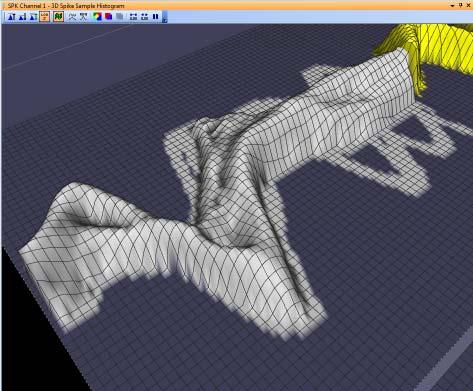
339 Release

340 10 User Interface Views and Features So far, the SSH3D has shown each unit s histogram separately. If you click Combine unit surfaces, all the units (and the unsorted unit) are shown superimposed on each other: When Combine surfaces is enabled, the next two buttons allow you to control the degree of transparency of the surfaces, allowing you to see through the outer histograms: 328 OmniPlex D Neural Data Acquisition System

341 The rightmost three buttons can be used to make the animated histograms update more slowly, faster, or to pause the animation. The fastest update rate will most closely follow changes in the firing rates of the displayed units, while a slower update rate tends to smooth out short-term fluctuations in activity. Note that the Pause button here is independent of the Pause button in the main PlexControl toolbar, so that the SSH3D view can be paused without affecting any other displays. Note that the spike Show Filter in the main PlexControl toolbar also affects the SSH3D view. For example, setting the Show Filter to Sorted causes only sorted spikes to be displayed in the SSH3D: Release

342 10 User Interface Views and Features The other Show Filter modes have analogous effects, e.g. Selected Unit + Unsorted: 330 OmniPlex D Neural Data Acquisition System

343 The SSH3D provides intuitive visual feedback about the quality of unit definitions and the relative activity of the different units on a channel. The unit displayed in green above is a good example of what a well-defined unit might look like, with a Gaussian distribution centered on a well-defined spine corresponding to the mean waveform. Note that in stereotrode and tetrode modes, the SSH3D currently only displays the first channel of each stereotrode or tetrode. Release

344 10 User Interface Views and Features 10.5 Channel Ranking The channel ranking feature allows the order of display in the multichannel spike, spike-continuous (SPKC), wideband (WB), and field potential (FP) views to be determined by one or more selected criteria. For example, channels can be ranked such that the channel(s) with the largest number of sorted units is/are displayed first. This can help draw your attention to interesting channels and reduces display clutter, especially at higher channel counts and/or if you have a significant number of inactive channels. In its simplest form, channel ranking can be used to place all disabled channels last in display order. By default, disabled channels are displayed like this: Click on the channel ranking button in the multichannel spike window s toolbar to enable channel ranking: 332 OmniPlex D Neural Data Acquisition System

345 With channel ranking enabled, disabled channels are pushed to the end of the display: Release

346 10 User Interface Views and Features The WB, SPKC, and FP continuous views will display their channels in the corresponding order (channels 1-27 are not visible here but are in normal order above channels 28-32): Click the Channel Ranking button again to return to the original unranked channel order. Note that channel ranking does not affect the data itself, the numbering or order of channels in recording files, clients, etc. It is purely an option for organizing the multichannel displays. Also note that the channel ranking is always a function of the channels in the SPK source; for example, if you disable different channels in the SPK and FP sources, the disabled SPK channels will determine the channel ranking. Channel ranking can be based on criteria other than (or in addition to) channels disable status. To see the available ranking options, click on the Display Options button in the spike window toolbar: The Display Options dialog is displayed, with the channel ranking options in the upper area as highlighted below: 334 OmniPlex D Neural Data Acquisition System

347 Arrange Channels in Rank Order has the same effect as the toolbar button, i.e. you can use either to toggle channel ranking on and off. Apply Ranking to Associated Continuous Views determines whether the channel ranking in the multichannel spike (SPK) window is applied to the WB, SPKC, and FP views. The Ranking Criteria dropdown list allows you to use additional criteria in determining the channel ranking. None means that no additional criteria are used, and only disabled channels determine the ranking. The remaining criteria are based on the most recent spike snapshot, so you must take a snapshot before using them. Firing rate is the per-channel mean firing rate, within the snapshot. For example, for the default 500 spikes per channel snapshot, the mean firing rate of each channel would be: MeanRate[channel] = 500 / (TimestampOfLastSpike[channel] TimestampOfFirstSpike[channel]) TotalSpikeEnergy for a channel is the sum of the individual spike energies for all spikes in the snapshot, where a spike s energy is defined as the sum of its squared waveform sample values. If different channels have the same number of spikes in their snapshots, the respective total spike energies will depend entirely on the relative spike energies. If different channels have different numbers of spikes in Release

348 10 User Interface Views and Features their snapshots, either because the snapshot was taken by time instead of by count, or if one or more channels snapshots timed out before their count was reached, then the total spike energies will depend on both the spike energies and the number of spikes in the snapshot. Number of units is the number of sorted units on each channel. The three remaining criteria are based on number of units first, and then within channels that have the same number of units, firing rate or total spike energy are used as a secondary ranking criteria. For example, Number of units, then spike energy would assign the highest ranking to the channel with the most sorted units and the largest spikes. Note that channel ranking is not dynamically updated, i.e. channels do not move around in the multichannel display in real-time as their firing rates or number of sorted units change. In the case where disabled channels are displayed last but no other ranking criteria are being used, you can refresh the display order by clicking the Channel Ranking button twice, to disable and then re-enable ranking. For cases where criteria based on the spike snapshot are being used, you must take a new spike snapshot before toggling the ranking off and then back on. When the ranking is re-enabled, it will use the most recently taken spike snapshot. 336 OmniPlex D Neural Data Acquisition System

349 10.6 Advanced User Interface Features The basic features of the OmniPlex D System user interface are described in the main body of this user guide. The following more advanced features are handy for users who wish to more extensively customize the layout of views and toolbars in PlexControl. Floating a window If you place the cursor on the title bar of a window, hold down the left button and drag, you will undock that window, and any tabbed views that are contained within it. If you then release the window while it is not attached to the edge of any other window, it will become a floating window that covers the windows beneath it. Here is an example: Release

350 10 User Interface Views and Features 338 OmniPlex D Neural Data Acquisition System

351 Docking a window As you are dragging a window, you will see sets of blue arrows appear at the four sides of the main PlexControl window (indicated by red circles below), and a four-way arrow in the center of the nearest window (indicated by a red square below). Release

352 10 User Interface Views and Features If you move the cursor to any of the four outer arrows, the window you are dragging will be docked to that edge. For example, if we dock the window to the right edge: We could then use the splitter bars to resize the windows, within this layout: 340 OmniPlex D Neural Data Acquisition System

353 On the other hand, if we release the cursor within one of the four arrows in the four-way arrow, the window will dock to that edge, but nested within that specific window, as opposed to the outer, main PlexControl window. For example: Release

354 10 User Interface Views and Features If you drag a window and release while the cursor is in the center of the four-way arrow set, then the dragged window will be added as a tab within the window. This is particularly useful in that you can drag an individual tab from one window into another. For example, we could drag the Activity window tab from the bottom-right window containing the continuous views, into the window which contains the multichannel spike and PCA views: 342 OmniPlex D Neural Data Acquisition System

355 Sometimes it requires a bit of thought and experimentation, but virtually any window layout can be achieved by a sequence of these operations. Release

356 10 User Interface Views and Features 10.7 PlexControl Keyboard Shortcuts The following keyboard shortcuts can be typed as either upper or lower case characters. T: Toggles display of the currently selected view's toolbar N: Go to the next channel P: Go to the previous channel O: Display the currently selected view's Options dialog S: Toggles display of snapshot versus live data space: Redraw view 344 OmniPlex D Neural Data Acquisition System

357 Plexon Inc Chapter 11 Saving Settings, Startup/Shutdown and Troubleshooting 11.1 Step by Step: Saving and Loading PlexControl Settings Step by Step: Automatically Maintaining Compatible Sets of PXS and PXC Files Starting and Shutting Down Server and PlexControl Interpreting LEDs on AMP LINK and DATA LINK Cards Troubleshooting Startup Problems Step by Step: Resetting All OmniPlex D System Options to Defaults Release

358 11 Settings, Startup and Troubleshooting 11.1 Step by Step: Saving and Loading PlexControl Settings 1 At any time, you can save the settings of all parameters in PlexControl (gain, thresholds, sorting parameters, etc) to a settings file, so that you can restore them later. To do this, simply click the Save button in the toolbar:. Note: Setting the gain is applicable to DigiAmp subsystems, not DHP subsystems. 2 Specify a filename using the standard Windows Save dialog. Note: PlexControl settings files have the extension.pxc. 346 OmniPlex D Neural Data Acquisition System

359 3 To load a previously saved pxc file, you can use either the Open or Open Most Recently Saved buttons in the toolbar: Note that you must stop data acquisition before loading a pxc file, and start data acquisition again after the file has been loaded. However, you do not have to stop data acquisition to save the current settings to a pxc file Step by Step: Automatically Maintaining Compatible Sets of PXS and PXC Files Settings in the OmniPlex D System are saved in two files: Server saves its topology and settings in a PXS file, and PlexControl saves its settings in a PXC file. For many users, a single PXS is used, and only the PXC file changes from experiment to experiment. However, other users use a number of different PXS files, and the issue of PXS/PXC compatibility arises. Specifically, if a PXC file was created while one PXS file was loaded in Server, but at later date, the same PXC file is loaded while a different PXC file is loaded in Server, incompatibilities, some difficult to detect, can occur. If your usage includes such mix and match scenarios, you may wish to enable a set of options in the OmniPlex D System which will automatically save your PXC and PXS files so that you know that you have a compatible pair of settings files 1 To enable PXS auto-save in Server, select Global Options from the Configure menu: Release

360 11 Settings, Startup and Troubleshooting 2 Enable Automatically save pxs when recording ends. 3 Click OK. 4 In PlexControl, select Global Options from the Configure menu: 348 OmniPlex D Neural Data Acquisition System

361 5 Select the Recording Files tab and enable Auto-save pxc. Now, each time that you record a plx or pl2 file, the current settings in Server and PlexControl will automatically be saved as XXX.pxs and XXX.pxc, where XXX is the name of the plx/pl2 file. In this scheme, for each plx/pl2 file you record, PlexControl will create three files with the same name, but with the extensions.plx/pl2,.pxc, and.pxs. If you later wish to run another experiment using the same settings as a previous session, you can load the corresponding pxs and pxc files in Server and PlexControl respectively Starting and Shutting Down Server and PlexControl There are a few best practices to keep in mind regarding the sequence in which Server and PlexControl are started and shut down. The recommended startup sequence is to run Server, wait for the initialization sequence to complete (indicated by the green progress bar at the bottom of the Server window), then start PlexControl, then start data acquisition. It is possible to first run PlexControl, which will then automatically start Server before allowing you to continue; however, if this method ever fails, you should fall back to the recommended sequence. When you are completely finished with the system and want to shut down the OmniPlex D System, the recommended sequence is to stop data acquisition from PlexControl, then close PlexControl, then close Server. In other words, the shutdown sequence is the reverse of the startup sequence. Release

362 11 Settings, Startup and Troubleshooting Closing and Opening Server (Applicable with DigiAmp Subsystem) When the Server application is closed (i.e. you exit to Windows), all data acquisition is stopped and the power to the DigiAmp Amplifier is turned off. The blue link cable between the AMP LINK card in the chassis and the DigiAmp Amplifier can then be safely unplugged. You should never plug or unplug the blue link cable while Server is open, even when data acquisition is stopped. You can verify the DigiAmp power status via the row of three green LEDs on the AMP LINK card in the chassis; if all three LEDs are on, power to the DigiAmp Amplifier is on; if only the leftmost LED is on, power to the DigiAmp Amplifier is off, and the cable can be plugged or unplugged. Note: If you are connecting the blue link cable to the DigiAmp or MiniDigi unit or the AMP LINK card in the chassis, make sure the red markings on the cable connectors line up before inserting the cable. Grasp the connector and push straight in. To unplug the cable, grasp the connector and pull straight out. See the caution statement below. The headstages can only be powered when the AMP LINK power to the DigiAmp Amplifier is on, as indicated by the three green LEDs. Of course, the HST PWR toggle switch on the DigiAmp Amplifier must also be on to enable the headstage power.. CAUTION Handle the blue cable correctly to avoid damage =Do not pull on the blue cable itself, and do not twist the connector. =Never bend or kink the blue cable. =Never plug/unplug the blue cable if the Server application is running. Closing and Opening Server (Applicable with DHP Subsystem) When the Server application is closed (i.e. you exit to Windows), all data acquisition is stopped and the power to the DHP unit is turned off. The blue link cable between the DATA LINK card in the chassis and the DHP unit can then be safely unplugged. You should never plug or unplug the blue link cable while Server is open, even when data acquisition is stopped. You can verify the DHP unit power status via the row of three green LEDs on the DATA LINK card in the chassis; if all three LEDs are on, power to the DHP unit is on; if only the leftmost LED is on, power to the DHP unit is off, and the cable can be plugged or unplugged. Note: If you are connecting the blue link cable to the DHP unit or the DATA LINK card in the chassis, make sure the red markings on the cable connectors line up before inserting the cable. Grasp the connector and push straight in. To unplug the cable, grasp the connector and pull straight out. See the caution statement above. The headstages are powered when the red PWR LED on the DHP unit is lit. 350 OmniPlex D Neural Data Acquisition System

363 Shutting Down and Reopening PlexControl (Applicable to All OmniPlex D Systems) You will find that if you shut down PlexControl without first stopping data acquisition, data acquisition continues to run in Server, which is expected. If you now re-open PlexControl, it will automatically reconnect to Server while data acquisition is running, and continue displaying incoming data as it did before you shut it down. However, this has the potential to cause occasional problems, particularly at high channel counts. Therefore, it is not recommended that you make a habit of leaving Server running without PlexControl attached to it. As a general rule, when you are done using PlexControl, you should also shut down Server. Release

364 11 Settings, Startup and Troubleshooting 11.4 Interpreting LEDs on AMP LINK and DATA LINK Cards This section explains how to interpret the LEDs on the front panel of the AMP LINK and DATA LINK cards. Note: AMP LINK cards are present in systems with the DigiAmp or MiniDigi subsystem. DATA LINK cards are present in systems with the DHP subsystem. The LEDs are the same on these two cards. The term blue box below refers to the DigiAmp, MiniDigi or DHP unit, as applicable. LED1 (green) Power LED2 (green) Power to blue box LED3 (green) Communication lock (with blue box) OK LED4 (orange) Sampling clock LED5 (orange) Sampling status LED6 (orange) (internal use) The LEDs can be interpreted as described below for typical system states, where + means ON (fully lit) means OFF (not lit) * means partly lit (lit but dim) Server not running: Server started, but acquisition stopped: Data acquisition running: 352 OmniPlex D Neural Data Acquisition System

365 11.5 Troubleshooting Startup Problems If you ever encounter a situation where data acquisition fails to start, and/or you receive any error message from Server, the first thing to try before contacting Plexon support ( or support@plexon.com) is to exit from PlexControl and Server, check all cables and power, and restart the OmniPlex D System. If this does not help, use the rocker switch on the back panel of the chassis to turn the power off and then back on (never do this while the OmniPlex D System is running!), then reboot Windows and try again. However, in most cases where the problem is an unplugged cable, wrong type of DigiAmp Amplifier, etc, Server will display an error message informing you of the problem. Problems involving incorrect or inconsistent application settings can often be solved with the software reset procedure described in the next section. Release

366 11 Settings, Startup and Troubleshooting 11.6 Step by Step: Resetting All OmniPlex D System Options to Defaults If you ever need to reset all PlexControl and Server options to their defaults, use the following procedure. The one setting that will not be reset is the pxs file which is auto-loaded by Server; however, if you want to prevent the last-loaded pxs file from auto-loading in Server, hold down the Ctrl key while starting Server. The reset procedure can be useful for troubleshooting, or if you simply want to ensure that you are starting from scratch, without carrying over any settings changes from a previous OmniPlex D System session. To reset all software options and settings in both PlexControl and Server: 1 Stop data acquisition as described previously. 2 In PlexControl, select the Reset All Options to Defaults command: 3 You will be asked to confirm the reset: 354 OmniPlex D Neural Data Acquisition System

367 4 Click Yes to confirm the reset. You will be prompted to shut down PlexControl: 5 Click OK, then close PlexControl (but do not restart it yet). 6 In Server, select the Reset All Options to Defaults command: Release

368 11 Settings, Startup and Troubleshooting 7 You will be prompted to confirm the reset: 8 Click Yes to confirm the reset. You will be prompted to shut down Server: 9 Click OK, then close Server. 10 Run Server and then PlexControl as usual. All software options and user interface layouts are now restored to their default settings. 356 OmniPlex D Neural Data Acquisition System

369 Plexon Inc Chapter 12 Additional Features 12.1 Audio Monitoring of Wideband or Spike Continuous Signals Digital Referencing Channel Mapping Thresholding Configuration Options Spike and Continuous Data Width Export to External Clients Release

370 12 Additional Features 12.1 Audio Monitoring of Wideband or Spike Continuous Signals The OmniPlex System supports online monitoring of the currently selected wideband (WB) or spike-continuous (SPKC) channel using the standard audio outputs of the computer on which the OmniPlex software is running. You may find it useful to listen to the live signal as an aid to electrode placement and for ongoing monitoring of spiking activity once electrodes have been positioned. To use this feature, you can listen to the audio using the speaker built into the computer, but for better quality you can plug headphones or external speakers into the audio output jack on the front or rear of the computer. The output jack will typically be marked with an icon of a pair of headphones or a speaker, or an arrow pointing outward from the jack. You can use either mono or stereo headphones or speakers, but the audio will be mono in either case, since you are listening to a single channel. Note: Be sure to check that the audio is not muted in the Windows audio control panel or mixer. Enable audio monitoring To enable audio monitoring and to choose wideband or spike-continuous monitoring, stop data acquisition, right-click on the Spike Separator in Server, and select Edit Device Options. In the Device Options dialog, select the desired audio monitoring option and click OK. 358 OmniPlex D Neural Data Acquisition System

371 When you start data acquisition, the selected monitoring option is enabled. When you select a channel in PlexControl, the corresponding WB or SPKC channel is automatically selected for audio monitoring. Helpful tips for using audio monitoring In most cases, you will probably want to monitor the spike-continuous (SPKC) signal, since field potential signals (i.e. frequencies below the spike band) tend to have poor audibility and are not very informative. The option to monitor the unfiltered wideband (WB) signal is provided primarily for users who wish to use an external equalizer to do custom filtering of the audio signal. Note that due to the constraints of the computer s audio output subsystem, it is possible that you may occasionally hear a very brief dropout or glitch in the audio. Also, the built-in PC audio may add a small amount of coloration or distortion, relative to the signal which is processed and recorded by the OmniPlex System. If you find the audio quality inadequate, try using the audio output jack on the rear panel of the computer, as in some cases this provides a cleaner signal. The above caveats should not be problematic in normal use, but it is important to keep in mind that the audio output is only intended for live monitoring, and is not necessarily suitable for recording or analysis. Release

372 12 Additional Features 12.2 Digital Referencing Overview Digital referencing can be configured on a per-channel basis for continuous spike (SPKC) channels and/or field potential (FP) channels. For either source, the referencing (digital subtraction of sample values) is performed immediately before the filtering operation, and consequently for the FP source, before the post-lowpass downsampling. In effect, two separate copies of the original wideband (WB) signal are subjected to independent referencing before being passed to the spike separator and FP separator. This ensures that there is no unwanted interaction between the referencing operation and the chosen filters, and that it is performed at the full 40 khz wideband sampling rate for maximum precision Configuring referencing in PlexControl Digital referencing is controlled via the multichannel Properties Spreadsheet in PlexControl. The two columns "DRef SPKC" and "DRef FP" display the digital reference settings for each channel of the SPKC and FP sources: Determine which channel you wish to use as a reference, typically by selecting a channel where unwanted artifacts are clearly present but very few spikes are seen. Select this channel number in the DRef column(s) in the rows corresponding to the channels which are to use this reference. Clicking on a cell displays a dropdown list of the available reference options (the CAR and CMR options will be described later): 360 OmniPlex D Neural Data Acquisition System

373 The number in the dropdown list is the actual channel (within the same source) which is to be used as a reference for the selected channel. Remember that you can use the right-button menu functions to quickly set a series of channels to the same reference channel. For example, to set five successive channels to all use channel 17 as their reference, set the topmost to channel 17, then drag-select the channels below it and use Set All Selected Channels Like Topmost Selected Channel. Release

374 12 Additional Features The selected channels are all set the same reference channel as the topmost channel: The default reference setting of None indicates that no referencing is to be performed on that channel. There a few simple rules to keep in mind. You cannot reference a channel against itself; there is no valid reason to do so (the result is guaranteed to be exactly zero, since the subtraction is in the digital domain), and you will usually want to be able to monitor the reference signal. If you use one of the right-button functions to set a group of channels to the same reference, and the reference channel is within the range of channels, it will be automatically skipped and its reference set to None, to prevent self-referencing. Also, a channel which is being used as a reference for other channels cannot itself be referenced to another channel - its reference must be set to None. References within the FP source are assigned in exactly the same way as for SPKC channels. However, you should be cautious when referencing FP channels, since in many cases the field potentials can be attenuated by referencing, due to the same signal being picked up by more than one electrode. You should use the SPKC and FP displays to monitor the effects of referencing, to verify that artifacts are being reduced or removed, while not harming the signals of interest. Note that no matter what referencing you apply to SPKC and/or FP channels, the wideband (WB) channels are unaffected. By recording the wideband channels, you can ensure that you have a record of the original signal, including artifacts, which you can later compare against the results of referencing, possibly apply offline referencing to, etc. 362 OmniPlex D Neural Data Acquisition System

375 Common average referencing (CAR) and common median referencing (CMR) In addition to standard referencing, where signals are subtracted pairwise (i.e. channel j is subtracted from channel k) in either the analog domain or digitally, the OmniPlex D System supports two additional methods of digital referencing which combine multiple channels to form a composite reference signal which is then subtracted to remove or reduce unwanted components. The basic idea of both CAR and CMR is that if many signal channels are averaged together, the averaged signal being the result of averaging corresponding sample values across channels, then artifact signals that are the same across all channels (such as AC power line noise) will "survive the averaging" in the reference signal, whereas components unique to each channel, such as spikes, will tend to "cancel out" and have a mean near zero. The difference between CAR and CMR is that with CAR, the mean of sample values at each sample time is used as the reference signal, whereas with CMR, the median is used. In many cases, CMR will give results that are more robust in the presence of amplitude outliers, i.e. it will produce a better reference signal. However, the choice of standard digital referencings versus CAR versus CMR is data-dependent and should be evaluated on a case by case basis. To select a channel for CAR (or CMR), select CAR (or CMR) from the channel's drop-down list in the Properties Spreadsheet. Notice that you have the option of selecting up to four independent CAR groups and up to four independent CMR groups simultaneously. If you are considering using multiple CAR or CMR groups, first read the discussion below Important considerations for using multiple CAR and CMR groups. Release

376 12 Additional Features Selecting and Monitoring CAR/CMR (for single CAR and CMR groups) You can select any number of channels to be included in CAR and/or CMR, although it is recommended that for best results, you use only one or the other method, and include as many channels as is practical, in order to achieve a good average or median reference signal. Note than unlike conventional referencing, the channels that are selected for CAR or CMR are both used to form the reference signal, and this signal is then subtracted from all the selected channels. Since the common average or common median will be subtracted from all CAR/ CMR channels, the OmniPlex D System provides a facility for monitoring and recording the CAR/CMR composite reference signal. If you designate a channel's reference as CARMon or CMRMon, that channel's original signal will be replaced by the actual CAR/CMR signal which is being subtracted from the channels whose reference is CAR or CMR respectively. For example, you can locate a channel which is otherwise unusable (e.g. due to a bad electrode) and designate it as the CARMon or CMRMon channel; the common average and common median reference signals can then be viewed in the SPKC or FP display, and recorded if desired. Alternately, you could use a standard procedure such as always allocating the last channel in SPKC/FP as the CAR/CMR monitor channel. Here is a "kitchen sink" example which should give some idea of the flexibility of this scheme; in practice, you would be unlikely to need such a complex set of references in a system with only 32 channels. Note that each non-car/cmr channel which is being used as a reference (SPKC channel 4 and FP channels 3 and 7) has its own reference set to None, as required. 364 OmniPlex D Neural Data Acquisition System

377 Important considerations for using multiple CAR and CMR groups When you have multiple CAR groups, the channels within each CAR group (e.g. CAR3) are averaged together and that average is subtracted from only the channels of that CAR group. Likewise, the sample-by-sample median of the channels within each CMR group (e.g. CMR4) is calculated and that median is subtracted from only the channels of that CMR group. Each CAR and CMR group can have an associated monitor channel. Any SPKC or FP channel can be assigned to any of the CAR or CMR groups, and the CAR and CMR groups are completely independent between SPKC and FP. For example, you could define one CAR group and three CMR groups on the SPKC channels, but two CAR groups and one CMR group on the FP channels. Defining more than one CAR and/or CMR group can be useful in cases where various subsets of channels each exhibit unique common noise or artifacts. For example, electrodes from one headstage may be implanted in a different part of the brain than another headstage, or multiple types of electrodes may be in use simultaneously, each with varying susceptibility to noise and artifacts. The user interface for defining multiple CAR/CMR groups and the associated monitor channels is a straightforward extension of the previous single-car / single-cmr scheme. When you click on a channel s entry in the DRef SPKC or DRef FP columns of the main Properties Spreadsheet, you will see the choices shown in the image below. Release

378 12 Additional Features For each channel, you can select a CAR group or a CMR group or a specific channel number as the reference. Select one of CAR, CAR2, CAR3, or CAR4 to assign a channel to CAR group 1, 2, 3, or 4 respectively. CARMon, CARM2, CARM3, and CARM4 are the corresponding CAR monitor channels. Select one of CMR, CMR2, CMR3, or CMR4 to assign a channel to CMR group 1, 2, 3, or 4 respectively. CMRMon, CMRM2, CMRM3, and CMRM4 are the corresponding CMR monitor channels. Selecting a specific channel number as the reference (1, 2, 3 n) simply subtracts that specific channel, rather than using common average referencing or common median referencing. In addition to the usual caveats about the use of CAR/CMR, using multiple CAR/ CMR groups can require additional caution. For the same overall channel count, defining more than one group implies that each group will contain fewer channels than if a single group were used, but it is important that each group contain enough channels that the average or median reference signal contains only artifacts and not identifiable spikes. The most important tool for ensuring that digital referencing is being applied appropriately is the monitor channel for each group. Each monitor channel should display artifacts, not spikes, and the artifacts on each monitor channel should be different than the other monitor channels; if the artifacts are the same on different monitor channels, this indicates that too many referencing groups have been defined, and you will in fact achieve better results by defining fewer groups, since more channels will then be included in the average or median of each group, helping to average out the spikes and to emphasize the artifacts. Remember that by recording the monitor channel(s), you are recording what is being subtracted out from the channel in each referencing group and you could potentially apply your own offline post-processing to add the reference signal(s) back to the channels in the corresponding groups and thereby reconstitute the original, unreferenced signals. 366 OmniPlex D Neural Data Acquisition System

379 12.3 Channel Mapping Channel mapping allows users of electrodes with nonstandard or inconvenient physical channel numbering, e.g. silicon probes, to map (renumber) the channels, such that the original physical channel numbering is hidden from the OmniPlex D System, without the use of custom adaptors or cables which were previously required. Note that currently only neural channels can be mapped; channels such as digital input and auxiliary analog (AuxAI) channels are not affected by channel mapping in any way. The OmniPlex D System channel mapping supports an arbitrary one-to-one mapping (renumbering) of electrode channels (also referred to as input channels) and the OmniPlex D System channels (also referred to as output channels). Each input channel must map to exactly one output channel, and vice versa. A channel mapping is specified by loading a cmf file (channel mapping file) in the OmniPlex Server. Once a cmf is loaded, it remains in effect until it is either manually disabled, a different pxs (topology) file is loaded or created in Server, or Server is started without a pxs file. You must close PlexControl before loading a new channel mapping file or disabling channel mapping in Server Creating a cmf file A cmf file is a simple text file which you can create using Windows Notepad or any other text editor which can create plain text files. After creating the file in an editor, renaming the file extension from.txt to.cmf will make the OmniPlex D System recognize it as a channel mapping file. Here is an example of a typical cmf file: Release

380 12 Additional Features This cmf is for a 16 channel system, so all channel numbers in the file are within the range Each line in this example specifies the mapping of one channel. The channel number on the left side of the = sign is the OmniPlex D System channel number as seen in PlexControl, in recording files, clients, etc. The channel number on the right side of the = sign is the original physical electrode channel number. In other words, the mapping commands are of the form: outputchannelnumber = inputchannelnumber or to put it another way: visiblechannelnumber = hiddenchannelnumber For example, say that the original electrode device was a 1D linear array probe, and the actual physical electrode channel numbers, starting from the tip of the probe, were the following: [probe tip] 9, 14, 6, 10, 4, 12, 2, 11, 13, 15, 3, 7, 1, 16, 8, 5 [probe top] but what you would like to see in the OmniPlex D System is a convenient list of uniform, increasing channel numbers like this: [probe tip 1, 2, 3, 4, 5, 6, 7, 8, 9, 10, 11, 12, 13, 14, 15, 16 [probe top] The above cmf file will accomplish this channel renumbering. In actual use, you will need to consult the documentation for your electrodes, or contact the manufacturer, to determine the electrode channel numbering, i.e. the device pinout. In a case such as the 1D probe example above, it may be obvious what the most useful channel mapping is; in other cases, where the electrodes are arranged in a complex geometry, an appropriate mapping may be a matter of preference, or there may be considerations unique to your experiment or data analysis. For example, if you are using a probe with multiple tetrode sites along a shank, you should assign consecutive channel numbers to the four channels within each tetrode, such that the tetrodes appear in the OmniPlex D System as channels 1-4, 5-8, etc. In many cases, a cmf file similar to the one above will be all that is necessary to define the desired mapping. However, the cmf file supports additional functionality that can make the definition of certain types of mappings easier. If you like, you can skip to Section , Loading a cmf file in the OmniPlex D System on page 373 on a first reading, and read about the additional features later. 368 OmniPlex D Neural Data Acquisition System

381 Default mapping In the above example, we explicitly specified the mapping for every single channel. This was because, as in many real-world cases, every channel on the device has to be renumbered. However, imagine that we have a probe or array where only the first eight channels have "inconvenient" physical channel numbers, and the last eight channels are numbered 9 through 16 as with a "normal" set of electrodes. The corresponding cmf might look something like this: 1=7 2=5 3=6 4=2 5=7 6=3 7=1 8=4 9=9 10=10 11=11 12=12 13=13 14=14 15=15 16=16 In other words, the last eight channels are to retain their original channel numbers. In a case like this, you need only list the channels that require actual mapping; all other channels are assumed to be unchanged: 1=7 2=5 3=6 4=2 5=7 6=3 7=1 8=4 Release

382 12 Additional Features Range mapping In some cases, you may wish to renumber contiguous blocks of channel numbers, which can be done with a range mapping: 1..4= = = =5..8 The notation 1..4 means channels 1 through 4, and likewise for the other channel ranges shown. For example, the range mapping 1..4=9..12 has the same effect as the following series of mapping commands: 1=9 2=10 3=11 4=12 You can see that the above cmf commands are in effect permuting four-channel blocks within a total of 16 channels. Swapping the first 32 channels and the last 32 channels in a 64 channel system could be done with these mappings: 1..32= =1..32 Note that you can use a combination of single-channel and range mappings within the same cmf file; for example: 1..4= =7 6=5 7=8 8= = =16 14=13 15=14 16= OmniPlex D Neural Data Acquisition System

383 Formatting and comments When the OmniPlex D System reads a cmf file, it ignores all spaces within each line of the file, so that the following commands are all equivalent: 1..32= = = = You can insert a comment line by using either ";" as the first character of a line, or "//" as the first two characters. Blank lines are also allowed. For example: ; Mapping file for MySiliconProbe ; July 19, 2013 // the next two lines are range mappings 1..4 = = 1..4 // these are single-channel mappings 5=7 6=5 7=8 8=6 13=16 14=13 15=14 16=15 However, note that you cannot currently put a comment on the same line as a mapping command: 1..4 = // this comment is illegal Release

384 12 Additional Features Overwriting mappings and strict mode By default, the OmniPlex D System allows you to specify mapping commands in any order, as long as the final result maps every input channel to one and only one output channel. This can include sequences of mapping commands that overwrite, or partially overwrite, a previous mapping, for example: 1..32= = =10 42=42 The net effect will be to swap the first 32 and last 32 channels, except for channels 10 and 42, which will not be mapped. This is easier than writing out a full sequence of 64 single-channel mapping commands. However, in cases where you do not need to use overwriting, you may wish to disable it, to enable the OmniPlex D System to detect cases where an error in your cmf file results in a mapping command which unintentionally overwrites another mapping. If you add a line with the special keyword "strict" before any other mapping command in the cmf, the OmniPlex D System will disable support for overwriting and will report an error when a mapping command attempts to overwrite a previous mapping. strict 1..32= =1..32 // the next two lines will give errors when the cmf is loaded // since they overwrite the mapping of channels 10 and 42 10=10 42= OmniPlex D Neural Data Acquisition System

385 Loading a cmf file in the OmniPlex D System Once you have defined a channel mapping in a cmf file, loading the file in the OmniPlex Server puts the mapping into effect. To load a channel mapping file, first close PlexControl, if it is open. Next, go to Configure >> Global Options: The Global Options dialog is displayed: Release

386 12 Additional Features To enable channel mapping, click Apply a channel mapping to the neural data channels and then click the Load Mapping File... button to specify the desired cmf file: 374 OmniPlex D Neural Data Acquisition System

387 You should see a confirmation that the cmf was loaded successfully: In the above example, 16 of 64 channels will be mapped (renumbered), while the other 48 will not be affected. The channel mapping is now in effect and the original physical electrode channel numbers are no longer used in the OmniPlex D System user interface, in recorded data files, or in online client data. As far as an OmniPlex D System user is concerned, the original channel numbering is completely hidden. If for any reason you later need to identify which physical input channel corresponds to a given OmniPlex D System channel, for example when analyzing your data, you can refer to the cmf file as a record of the mapping that was in effect. Release

388 12 Additional Features If any errors are detected when the cmf file is read by the OmniPlex D System, an error message is displayed, such as: When an error is detected, the OmniPlex D System automatically temporarily disables channel mapping, to prevent an invalid mapping from being applied. After correcting the error in the cmf (by editing the file in Notepad, etc), you will need to re-enable channel mapping and load the file again. Once a cmf has been loaded without error, the OmniPlex Server will automatically load the mapping file every time it starts, until you do one of the following: Manually disable channel mapping in the Global Options dialog Load a different pxs file (topology) in Server Use the Topology Wizard to generate a new topology Start Server without auto-loading a pxs file, for example by holding down the CTRL key while launching Server If the OmniPlex D System automatically disables a channel mapping that was previously in effect, a warning message is displayed, for example: Channel mapping can also be automatically disabled if Server attempts to autoload a cmf on startup but the file has been deleted or corrupted since it was last loaded. 376 OmniPlex D Neural Data Acquisition System

389 You can easily confirm the channel mapping file that was auto-loaded by viewing Server's Messages window as it starts up: To change the mapping, simply display the Global Options dialog and follow the procedure previously described. Note that you must stop data acquisition and close PlexControl before loading a new channel mapping file or manually disabling channel mapping. Release

390 12 Additional Features 12.4 Thresholding Configuration Options To access the threshold options, first make sure that data acquisition is stopped, then right-click on the Thresholding device in the topology in Server and select Edit Device Options: 378 OmniPlex D Neural Data Acquisition System

391 The Thresholding Configuration dialog is displayed: Return to Zero Thresholding Option The thresholding option, Sigma must return to zero between spikes, can yield improved spike detection in situations where the signal to noise ratio is poor and/ or the threshold is set close to the noise level. Release

392 12 Additional Features By default, the spike detector re-arms ( starts looking for another spike ) after the end of each detected spike only after the signal level has dropped below the threshold level (i.e. towards zero); until this occurs, another threshold crossing (i.e. away from zero) by definition cannot occur. However, if the Signal must return to zero between spikes option is selected, a stricter rule for re-arming is used: the signal must not only drop below the threshold, it must actually return to zero before a subsequent spike can be detected. If the threshold is set conservatively, for example by using the system default autothresholding method (threshold at three or four sigmas from the mean or median), the difference between the two re-arming options will often be small. However, in cases where the threshold is set closer to the edge of the noise band on a channel, using the return to zero option can reduce the amount of false detection and premature triggering. Note that the return to zero option is currently only implemented for singleelectrode thresholding, not for stereotrodes or tetrodes Threshold Crossing Rate Limiting The OmniPlex D thresholding algorithm extracts waveform segments from continuous signal channels in the SPKC spike-continuous source, triggered by threshold crossings. In normal circumstances, when threshold values are set appropriately, and in the absence of excessive noise, the resulting waveform segments are valid action potentials, i.e. spikes. However, in atypical situations, such as signals containing high amplitude, high frequency noise, and/or thresholds that the user sets too close to zero, the system will still proceed to extract potentially large numbers of spikes at firing rates that are physiologically improbable. For example, with the default spike length of 800 microseconds, setting a zero threshold on background noise can result in a sustained firing rate of 1.25 khz per channel. In such scenarios, it would be more correct to refer to the threshold crossing rate rather than the firing rate, since neurons cannot fire at such rates for more than a fraction of a second, if at all. Whether due to incorrect threshold settings or intervals of unavoidable high amplitude noise, it is preferable to suppress these spurious noise spikes, so that they do not unnecessarily increase recording file size, clutter displays, increase the processing and memory requirements for online and offline analysis programs, or degrade system performance. The Threshold Crossing Rate Limiting option provides a method for automatically detecting the atypical situations described above and temporarily suppressing such physiologically unlikely threshold crossing rates. 380 OmniPlex D Neural Data Acquisition System

393 Note that rate limiting is enabled by default. You can completely disable it if you wish, although this is not recommended, especially with high channel count systems (96 channels or more). The default rate limit is proportional to the system channel count, ranging from 1500 Hz per channel at 48, 32, or 16 channels, down to 300 Hz per channel for a 256 or 512 channel system. Rate limiting is controlled by two parameters, the Mean per-channel rate and the rate evaluation interval (Evaluate rate every parameter). The default values for these parameters have been chosen to ensure that rate limiting is applied to the thresholding process only when pathologically high threshold crossing rates are detected, and you should understand the following description of how they affect rate limiting before modifying them Rate Limiting Example At an interval controlled by the rate evaluation interval parameter, by default every 250 ms, the rate limiter examines the total number of threshold crossings, summed over all spike channels, to determine the mean-per channel rate over the preceding evaluation interval. For example, if there are 128 spike channels and the total number of threshold crossings was 1078 over a 250 ms interval, the mean per-channel rate would be (1078 total spikes / 128 channels) / 0.25 sec = 33.7 Hz This is far below the rate limit of 600 Hz per channel, so no rate limiting will occur, and the spike data will be passed on to the sorter unchanged. Now consider the other extreme, the zero threshold in noise scenario previously described. If the total number of threshold crossings in a 250 ms interval was 39137, the per-channel rate would be: (39137 total spikes / 128 channels) / 0.25 sec = 1223 Hz This is more than double the 600 Hz rate limit, so starting with the next 250 ms interval, spikes will be automatically culled from the data stream as necessary to limit the firing rate to 600 Hz; in this example, approximately every other spike will be removed. Every 250 ms, the aggregate spike rate across all channels will Release

394 12 Additional Features be re-evaluated, and the number of spikes culled will be updated as necessary to stay within the rate limit. As soon as the aggregate spike rate drops below the limit, rate limiting immediately stops until an excessive rate is detected again. Note that even when rate limiting is being performed, any individual channel on which fewer than the maximum number of threshold crossings occur within an evaluation interval will not be affected. For example, if a brief burst of high frequency noise occurs on all channels, and therefore initiates rate limiting, but in the next 250 ms interval, only one channel s firing rate exceeds 600 Hz, no spikes on any other channel will be affected. Since rate limiting does not occur until the interval after the interval within which the excessive rate was detected, brief bursts (by default, up to 250 ms) of even physiologically implausible activity will be passed through without change, while protecting against sustained non-neural threshold crossing rates. When rate limiting is taking place, and spikes are being removed on one or more channels, a rate limiting indicator in the PlexControl status bar displays the rate limiting in effect: In this example, the spike rate is being limited to 75% of what it would be if rate limiting were not applied. In other words, 25% of the threshold crossings are being removed, implying that the mean crossing rate is approximately 600 Hz / 0.75 = 800 Hz. When the yellow Rate Limit indicator is not displayed, 100% of spikes are available. Again, remember that channels whose firing rate is less than the rate limit will not be affected. Remember that rate limiting has no effect in a situation when one, or a small percentage of channels have an excessive threshold crossing rate. It is intended only to suppress pathological firing rates when they occur across many channels simultaneously, for a period longer than the evaluation interval. 382 OmniPlex D Neural Data Acquisition System

395 Rate limiting has no effect on the latency of spikes, whether rate limiting is in effect or not. Rate limiting only affects spikes (waveform segments) and has no effect on continuous data. If you record the continuous wideband (WB) and/or spike-continuous (SPKC) sources, you will be able to apply appropriate thresholds and extract valid spikes from the recorded data offline, assuming that any rate limiting during the recording was the result of a too-low threshold, and not caused by excessive noise in the original analog signals Thresholding By Aligned Extraction By default, the OmniPlex D System uses a standard thresholding (spike extraction) algorithm which defines the time at which the spike waveform crosses (exceeds) the threshold as its timestamp. While this is a classic method of thresholding, it has some drawbacks. First, it means that as the threshold is raised or lowered, the threshold hits the spike at different points on a rising or falling edge, potentially resulting in the timestamp changing by one, two, or more sample positions. Another manifestation of the same effect is that spikes of different amplitudes will have slight timestamp offsets relative to each other. While the size of these timestamp errors or jitter is too small to cause problems in most spike train analyses, it does have a significant effect on spike sorting: it causes smearing of clusters in feature space. The basic problem with threshold timestamping is that it does not use an unambiguous feature (in time/voltage space) of the spike as the reference to which a timestamp is attached. The obvious choice for such a reference is the largest peak within the spike. The OmniPlex D System aligned extraction thresholding algorithm uses this approach. Release

396 12 Additional Features Here is an example of the difference between standard threshold crossing (top) and aligned extraction (bottom). Note how the waveform bundles and the corresponding PCA clusters are more well-defined when aligned extraction is used: Besides the improved timestamping accuracy and jitter reduction, the more welldefined clusters improve the performance of the automatic unit finding algorithm. 384 OmniPlex D Neural Data Acquisition System

397 Aligned extraction can be enabled in the device options for the thresholding device in Server: The first setting is standard thresholding, while the next two are two varieties of aligned extraction. The time of largest peak (same side as threshold) setting is recommended (as shown above), because typically you will set the threshold for a channel on the side where the larger-amplitude peaks occur. You must stop data acquisition before changing the thresholding mode. Note that there is one other change which you will probably wish to make when using aligned extraction. Due to the peak, rather than the threshold crossing, being used as the timestamp of spikes, the ratio of pre-threshold to post-threshold time tends to be different when aligned extraction is used; in other words, a longer prethreshold time is appropriate. As a typical example, the default the OmniPlex D System settings are a waveform length of 800 microseconds and a pre-threshold Release

398 12 Additional Features time of 200 microseconds; when aligned extraction is enabled, it is suggested that the pre-threshold time be increased to 300 microseconds. However, the correct values for waveform length and pre-threshold will be somewhat dependent upon the type and shape of action potentials that you are recording. You should ensure that the waveform length and pre-threshold are long enough to capture the features of the spike, without including unwanted noise and artifacts at the head or tail of the spike. 386 OmniPlex D Neural Data Acquisition System

399 12.5 Spike and Continuous Data Width Export to External Clients In the RASPUTIN Emulation Options dialog (see the diagrams below) you can select the resolution of the continuous and spike waveform data sent to online clients: 12 bits The system will encode all continuous and spike waveform data sent to online clients as signed 12 bit values within a 16 bit word. In other words, the raw unscaled sample values occupy a range from 2048 to This option should be selected if you need compatibility with legacy online clients which expect 12 bit values, as were used in the original Plexon MAP ( Harvey Box ) system. 16 bits The system will encode all continuous and spike waveform data sent to online clients as full 16 bit words, that is, full 16 bit resolution with sample values in the range to This provides an additional four bits (a factor of 16) more resolution than 12 bit values. Release

400 12 Additional Features Note: When 16 bit mode is enabled for data sent to external clients that are designed for processing 12 bit data, you must set the client programs to divide sample values by an additional factor of 16 (preferably in floating point, so as to take advantage of the four bits of additional precision) to maintain correct voltage scaling. CAUTION Client programs must scale 16 bit data correctly If you enable 16 bit mode for data sent to external clients, you must set the client programs to scale the sample values correctly. Otherwise, scaled voltages on the external client will be larger than the true values. Follow these steps to change the data width: 1 In the RASPUTIN Emulation Options dialog, select 12 bits or 16 bits for the data width. 2 Save the pxs file. 3 Shut down and restart the OmniPlex D System, start data acquisition, then run any client programs as usual. 388 OmniPlex D Neural Data Acquisition System

401 Plexon Inc Chapter 13 MultiPlex Multi-source View 13.1 Introduction Getting Started with the MultiPlex View Accessing Features in MultiPlex View Toolbar Commands Moving and Removing Channels Toolbar Commands Sweep and Magnification Controls Toolbar Commands Row Layout and Sizing Tools Toolbar Commands Show Scope Windows Toolbar Commands Customize Spike Displays Toolbar Commands Adjust Display of Ticks Toolbar Commands Spectrograms and Spectral Graphs Right-Click Menu Group Channels Right-Click Menu Move Selected Source Right-Click Menu Add/Remove Source or Channels Right-Click Menu Reset Spike Counts Right-Click Menu Draw Selected Channel s Ticks as Overlay MultiPlex View Options Dialog Scopes Fill Column in Fit Channels in Window Mode Vertical Splitter Limitations in MultiPlex View Keyboard and Mouse Shortcuts for the MultiPlex View Release

402 13 MultiPlex Multi-source View 13.1 Introduction This chapter describes the MultiPlex multi-source view and how to use it. The MultiPlex view allows you to view a customized set of spike, continuous, and event channels from any combination of sources, in any order. Channels are displayed in rows, as in the Activity view, but each row can contain any one of the three types of channels, and each type of row can be sized independently. Besides the rows of sweeping signal traces and/or ticks, an optional column of "scope" windows can be displayed to their left. For example, for a spike channel, where the main display shows spike ticks, the scope displays the waveforms for that channel, together or in individual unit windows. "Slow" continuous channels (sampling rate <= 5 khz) can be displayed as either signal traces or as spectrograms; when in spectrogram mode, the scopes for these channels display the associated spectral graph (FFT). Here is an example of a MultiPlex view. Many options are available for adjusting the way in which channels are displayed, for adding and removing channels, etc. Besides the flexible display configuration, there are other new visualization features such as rolling waveform variance envelopes, an oscilloscope-like spike display mode, and tracking of spectral peak frequencies. You can scroll through hundreds of channels of online spike, continuous, and spectrogram displays, with modest CPU usage. 390 OmniPlex D Neural Data Acquisition System

403 13.2 Getting Started with the MultiPlex View The MultiPlex view is automatically created when PlexControl starts up, like most other views: However, it is different in that by default it initially displays no channels. When you select the MultiPlex tab, a message is displayed in the middle of the empty window, prompting you to add channels. This can be done in two ways: 1 Checking a box in the MPX column of the main Properties Spreadsheet adds that channel to the MultiPlex view. Unchecking the box removes the channel from the MultiPlex view. You can add and remove channels at any time. Remember that you can make a source visible in the Properties Spreadsheet either by clicking on a view that is displaying that source, or by using the Previous Source / Next Source buttons in the main PlexControl toolbar to cycle through all the available sources, including sources like CinePlex events and keyboard events. Release

404 13 MultiPlex Multi-source View 2 Right-clicking on a channel in any spike, continuous, or activity view, and selecting Add Channel to MultiPlex View from the right-click menu. One exception to note is that from the Activity view, you can select and add spike channels using the right-click menu, but not event channels. However, you can use the Previous Source / Next Source toolbar buttons in the main toolbar to select the desired event source into the Properties Spreadsheet and then use the MPX column to add event channels. Using either method, each added channel results in a row being added to the MultiPlex view. TIP Use the keyboard and mouse shortcuts in MultiPlex view There are a number of keyboard and mouse shortcuts you can use to manipulate the rows in the MultiPlex display. See Section 13.20, Keyboard and Mouse Shortcuts for the MultiPlex View on page OmniPlex D Neural Data Acquisition System

405 13.3 Accessing Features in MultiPlex View The MultiPlex view has many commands that give you a great deal of control over the displayed channels and data. There are several methods you can use to access all of the MultiPlex view features. Some of the features are available in only one method, and some features are available by means of multiple methods. These methods are summarized in the following sections. Section , MultiPlex View Toolbar Commands on page 393 Section , MultiPlex Right-click Menu on page 394 Section , Options Dialog on page 395 Section 13.20, Keyboard and Mouse Shortcuts for the MultiPlex View on page 417 You should also familiarize yourself with the information in Section 13.19, Limitations in MultiPlex View on page MultiPlex View Toolbar Commands To view the toolbar commands, click the down arrow in the MultiPlex view header. Release

406 13 MultiPlex Multi-source View The uses of these toolbar commands are discussed in the following sections: Section 13.4, Toolbar Commands Moving and Removing Channels on page 396 Section 13.5, Toolbar Commands Sweep and Magnification Controls on page 397 Section 13.6, Toolbar Commands Row Layout and Sizing Tools on page 399 Section 13.7, Toolbar Commands Show Scope Windows on page 401 Section 13.8, Toolbar Commands Customize Spike Displays on page 402 Section 13.9, Toolbar Commands Adjust Display of Ticks on page 406 Section 13.10, Toolbar Commands Spectrograms and Spectral Graphs on page MultiPlex Right-click Menu You can access a wide range of MultiPlex commands by right-clicking anywhere in the MultiPlex view: 394 OmniPlex D Neural Data Acquisition System

407 As shown in the image above, some of the commands in the right-click menu display icons that are associated with toolbar commands, which signifies that those commands are available through both the toolbar and through the rightclick menu. Those commands function identically whether you access them using the toolbar or from the right-click menu. For a description of those toolbar commands, see the applicable sections in this chapter. Some of the commands in the right-click menu are available only through this menu, and they are discussed in the following sections: Section 13.11, Right-Click Menu Group Channels on page 409 Section 13.12, Right-Click Menu Move Selected Source on page 410 Section 13.13, Right-Click Menu Add/Remove Source or Channels on page 410 Section 13.14, Right-Click Menu Reset Spike Counts on page 411 Section 13.15, Right-Click Menu Draw Selected Channel s Ticks as Overlay on page Options Dialog One of the important features accessible from the MultiPlex toolbar and rightclick menu is the Options dialog. (It is also accessible by pressing the O key on the keyboard while the MultiPlex window is selected.) Several of the topics in this chapter will refer to the controls in this dialog. See Section 13.16, MultiPlex View Options Dialog on page 413. Release

408 13 MultiPlex Multi-source View 13.4 Toolbar Commands Moving and Removing Channels Channels are displayed in the order in which they are added, but changing this order is easy. Select a channel and, holding down the left mouse button, drag up or down to move the channel up or down in the list of channels. Alternately, you can do this by selecting a channel and then using the up-arrow/down-arrow keys while holding down Shift. In addition, there are toolbar and menu commands that move channels and sources (i.e. all the MultiPlex channels from the same source as the selected channel) to the top or bottom of the view. For example, these toolbar commands move the selected channel to the top or bottom of the display, or remove it from the view: Remove Selected Channel from Display Move Selected Channel to Bottom Move Selected Channel to Top There are other ways to remove channels from the display: You can delete a channel by selecting it and pressing the Delete key. The Remove All Channels from Display command in the MultiPlex rightclick menu resets the view to the empty state (a message box will ask you to confirm that you really want to remove all channels). Disabled channels are not displayed in the MultiPlex view. If a channel in the MultiPlex view is disabled from anywhere in PlexControl, it is automatically removed from the view. 396 OmniPlex D Neural Data Acquisition System

409 13.5 Toolbar Commands Sweep and Magnification Controls Sweep Controls The leftmost toolbar command is Erase, which clears the display. Sweep Faster and Sweep Slower adjust the speed of horizontal scrolling of the displayed data; they also affect the rate at which the data are updated. Erase Sweep faster Sweep slower Magnification Controls These tools give you direct control of the magnification factor. You can perform any of the following actions: Type in a new magnification factor and press the Enter key Use the spin controls (increase or decrease magnification by clicking the up or down arrow) Click the Reset Magnification button to reset the magnification to 1.00 Reset Magnification to 1.00 Magnification Factor Spin Controls Important considerations when managing MultiPlex magnification Magnification is slightly more complicated than in other views, since the MultiPlex view can contain channels from different sources. By default, changing the magnification using the spin controls changes the magnification on all spike and continuous channels in the view. If you hold down Ctrl or Shift while clicking the spin arrows, the behavior is as follows: Ctrl = change magnification for only the currently selected channel Shift = change magnification for all channels of the selected source (i.e. the source for the currently selected channel) A handy way to remember this is "C and S": Ctrl = Channel, Shift = Source. Using the mousewheel for magnification You can also adjust magnification using the mousewheel. See Section 13.20, Keyboard and Mouse Shortcuts for the MultiPlex View on page 417. Release

410 13 MultiPlex Multi-source View Auto-magnify Spikes and Continuous Auto-magnify commands Using these commands, you can let the system automatically adjust magnification. Auto-magnify spikes Auto-magnify continuous In practice, you may find that you don't need to manually adjust the magnification very often, but can use the auto-magnify tools instead. When you click on either of the above toolbar commands, all spike or continuous channels are monitored for a given interval (10 seconds by default, but this can be changed in the Options dialog) and then the magnification is set automatically on a perchannel basis. A handy shortcut is simply to press the 'A' key on your keyboard (note that the MultiPlex view must be selected first), which starts the automagnify procedure for all channels, both spike and continuous. Perform auto-magnify when adding a channel There is an option in the Options dialog to automatically perform an automagnify whenever you add a channel to the view: The last option, Respond to Magnification Chain Control from Other Views, causes magnification changes from other spike and continuous views to also adjust the magnification of the corresponding source in the MultiPlex view. 398 OmniPlex D Neural Data Acquisition System

411 13.6 Toolbar Commands Row Layout and Sizing Tools Fit Channels in Window Clicking the Fit channels in window command fits all the channels in the MultiPlex view into the window, so that you never need to scroll to see them all. However, to keep the view from becoming unusably crowded, the system limits the number of channels (rows) to 64; if there are more than 64 channels in the MultiPlex view, this command is disabled. Note that once you enable Fit channels in window, it is a mode that is in effect. If you add another 20 channels, it will still make everything fit in the window. If you only have one channel, it will expand that one channel to fill the full height of the window, which may not be the ideal appearance. If the layout appears awkward, consider whether you have Fit channels in window turned on, and whether it's appropriate for what you are trying to display Make All Rows the Same Height This command makes all rows in the MultiPlex view the same height Make Channels Taller/Shorter These commands make all the channels in the MultiPlex view (spike, continuous, and event) appear taller or shorter. Make all channels shorter Make all channels taller Release

412 13 MultiPlex Multi-source View Each of the commands in the image below applies only to a specific category of channels in the MultiPlex view. The S commands make all spike channels taller/shorter; The C commands make all continuous channels taller/shorter; the E commands make all event channels taller/shorter: Make spike channels taller/shorter Make event channels taller/shorter Make continuous channels taller/shorter Note that the default row heights are not the same Spike channels are the tallest and event channels are the shortest, since that works well in typical use. You can always use the above commands to size them any way you like. There is also a feature than currently can only be toggled from the Options dialog which automatically enlarges the currently selected channel to a specified percentage of its normal height; for example, the default value of 250% means that the selected channel is 2.5 times as tall as when it is not selected. Another option allows the currently selected channel to be automatically moved to the top row. The combination of these two options in effect "features" a channel in the MultiPlex view, without it "taking over" the entire window like the usual OmniPlex "double-click to zoom channel" functionality. Note that the latter option (When Channel is Selected in Other Views, Move to Top Row) only applies when a channel is selected from "outside" the MultiPlex view. (You actually wouldn't want selecting a channel in the MultiPlex view to automatically [and suddenly] pop it to the top row of the display.) Note: If you do want to move a channel to the top or bottom of the display, use the following commands: 400 OmniPlex D Neural Data Acquisition System

413 Note that there are also MultiPlex right-click menu commands for Move Selected Source to Top/Bottom, which act similarly to Move Selected Channel except that all the channels in the same source as the selected channel are moved to the top or bottom of the window Grouping Channels Move Selected Channel to Bottom Move Selected Channel to Top Two of the right-click menu commands affect the top to bottom order of all the channels in the MultiPlex view: Group Channels by Source and Group Associated Channels. For this information, see Section 13.11, Right-Click Menu Group Channels on page Toolbar Commands Show Scope Windows This command toggles the display of the column of "scope" windows to the left of the main channel rows. For example, with scopes off: Release

414 13 MultiPlex Multi-source View Scopes on, and with the spike channels made larger: The unit windows display the current relative number of spikes detected. There is a menu command for resetting the spike counts (see Section 13.14, Right-Click Menu Reset Spike Counts on page 411), and an option in the Options dialog for displaying raw counts instead of percentages (see Section 13.16, MultiPlex View Options Dialog on page 413) Toolbar Commands Customize Spike Displays These commands allow you to customize the spike and tick displays Show Units in Separate Windows This command toggles the display for a particular spike signal to show all units for the spike or to show only one individual unit belonging to the spike signal. For example, with separate unit windows off: 402 OmniPlex D Neural Data Acquisition System

415 With separate unit windows on: Row and Column Layouts for Unit Windows By default, the MultiPlex view automatically arranges the unit windows in rows and columns. However, these two commands allow you to force it to display the unit windows in rows or columns: Column layout for unit windows Row layout for unit windows For example, with separate unit windows and a row layout: Release

416 13 MultiPlex Multi-source View High-speed Update Mode This command toggles high speed updating mode ( scope mode ). When this mode is enabled, the spike waveform displays operate in a quasioscilloscope mode, where each new spike erases the one before it, but the most recent spike remains until another one is seen. This gives a result similar to using an external oscilloscope, one for each channel in the MultiPlex view. If you disable high speed updating, the display returns to the classic "accumulate and periodic erase" mode, with an erase time that you can set in the Options dialog Show Unit Variance This command toggles display of rolling variance envelopes. For example, with display of variance enabled: 404 OmniPlex D Neural Data Acquisition System

417 The shaded envelope indicates plus or minus N sigmas from the mean. The mean waveform itself is not displayed (it would clutter the display) but is by definition the centerline down the middle of the variance envelope. Both the mean and the variance are calculated from a moving window M spikes long, and incrementally updated on every spike. Both the length of the moving window (in spikes) and the distance of the variance envelope from the mean (in sigmas) can be set in the Options dialog. The basic idea is that a well-defined unit should have a tight variance envelope. For example, you can see that the unsorted units above have a large variance, as you would expect, since they are collections of dissimilar waveform shapes that may represent superpositions, artifacts, etc. You can think of the variance envelope as one kind of online sort quality metric - a tight variance envelope is the time domain equivalent of a tight, well-defined PCA cluster. Note that the variance envelope does not appear until [window length] spikes have fired on a unit after you enable variance envelopes, so depending upon firing rates, it may take a few seconds before the variance envelope is displayed. Release

418 13 MultiPlex Multi-source View 13.9 Toolbar Commands Adjust Display of Ticks Show ticks with amplitudes Show unit ticks on separate timelines The function of the Show unit ticks on separate timelines command is self explanatory. The Show ticks with amplitudes command causes ticks to be drawn not with uniform heights, but according to the peak positive and negative amplitude (bipolar amplitude) of each spike. Here is an example of all units being displayed on the same timeline, and with bipolar amplitude of the ticks enabled (Show ticks with amplitudes command selected): This image shows the units being displayed on separate timelines and with amplitudes enabled (Show unit ticks on separate timelines and Show ticks with amplitudes commands selected): 406 OmniPlex D Neural Data Acquisition System

419 13.10 Toolbar Commands Spectrograms and Spectral Graphs For "slow" continuous channels (sampling rate < 5 khz), there is an alternate display mode which shows a rolling spectrogram instead of the continuous signal, similar to the standard OmniPlex Spectral view, but with the sweep synchronized to the other channels in the view. This is enabled and controlled via the next three toolbar commands: Show Slow Continuous Channels as Spectrograms The Show Slow Continuous Channels as Spectrograms command toggles spectrogram mode on and off. For example, the following images show the MultiPlex display before and after clicking the Show Slow Continuous Channels as Spectrograms command for the channels FP001 and FP002: Release

420 13 MultiPlex Multi-source View If scopes are also enabled, then in spectrogram mode a spectral graph scope appears to the left of each spectrogram. As with the standard OmniPlex Spectral view, the spectral graph can be thought of as a vertical slice of the spectrogram at the current sweep time: The readout in the upper-right corner of each spectral graph indicates the frequency of the FFT bin with peak magnitude, continuously updated. For example, if you leave the inputs to the neural channels on your signals floating (disconnected), you may see a spectral peak at the 50 or 60 Hz power line frequency being picked up by the floating inputs, i.e. hum: The Increase/Decrease spectrogram amplitude commands control the amplitude scaling, and work the same way as in the main OmniPlex Spectral view: the red arrow scales up (more red, less blue), the blue arrow scales down (more blue, less red). Decrease spectrogram amplitudes (more blue) Increase spectrogram amplitudes (more red) 408 OmniPlex D Neural Data Acquisition System

421 13.11 Right-Click Menu Group Channels Two of the right-click menu commands affect the top to bottom order of all the channels in the MultiPlex view: Group Channels by Source and Group Associated Channels. For example, if you had the first two channels of WB, SPKC, SPK, and FP in the MultiPlex view, grouping them by source would yield this top to bottom order: SPK01 SPK02 WB01 WB02 SPKC01 SPKC02 FP01 FP02 On the other hand, grouping associated channels would produce this order: SPK01 SPKC01 WB01 FP01 SPK02 WPKC02 WB02 FP02 Note that unlike Fit Channels in Window, these are commands, not modes; they change the display layout when invoked, but you can then continue to change the row order with other commands and/or by manually dragging channels up or down in the list. There is currently no way to specify a different ordering of sources, or of associated channels when the above commands are used (e.g. perhaps you'd prefer the source order WB, SPKC, SPK, FP). However, grouping by source, followed by use of the Move Source to Top/Bottom command, can achieve the same effect. Release

422 13 MultiPlex Multi-source View Right-Click Menu Move Selected Source Move Selected Source to Top/Bottom moves all of the channels belonging to the source (that is, the same source as the selected channel) to the top/bottom of the MultiPlex View display. Note: For Move Selected Channel to Top/Bottom, see Toolbar Commands Moving and Removing Channels on page Right-Click Menu Add/Remove Source or Channels Add Associate Channels adds the parallel channels derived from the same wideband channel. For example, if you select SPK02 and click Add Associated Channels, channels WB02, FP02, and SPKC02 will be added if they are not already in the MultiPlex view. Remove Selected Channel from Display See Section 13.4, Toolbar Commands Moving and Removing Channels on page 396. Remove Selected Source from Display removes all channels belonging to the source (that is, the same source as the selected channel) from the MultiPlex View display. If you select Remove All Channels from Display, the system prompts you to make sure that is what you want to do. If you click OK, the system removes all channels from the MultiPlex view. You can display channels again by opening the Properties Spreadsheet and clicking the MPX checkboxes for the desired channels. 410 OmniPlex D Neural Data Acquisition System

423 13.14 Right-Click Menu Reset Spike Counts Reset Spike Counts sets the spike count(s) to 0 for all channels. Spike counts Release

424 13 MultiPlex Multi-source View Right-Click Menu Draw Selected Channel s Ticks as Overlay Draw Selected Channel s Ticks as Overlay only applies to event channels that are displayed in the MultiPlex view. The image below shows several event channels and two spike channels. For event channel KBD2, the user has selected Draw Selected Channel s Ticks as Overlay in the right-click menu. Therefore, the system extends the tick lines for KBD2, causing them to be overlaid on all the other channels in the MultiPlex view. Notice that the event channels KBD1, KBD3 and KBD4 have not been selected for overlay, so their tick marks are not extended. 412 OmniPlex D Neural Data Acquisition System

425 13.16 MultiPlex View Options Dialog The MultiPlex View Options dialog contains a number of options and settings that let you customize the default appearance of the data displayed in the MultiPlex view. You can access this dialog in several ways: From the MultiPlex toolbar From the MultiPlex right-click menu By pressing the O key on the keyboard while the MultiPlex window is selected In the image below, the default values are displayed. Release

426 13 MultiPlex Multi-source View Scopes Fill Column in Fit Channels in Window Mode The usual rule with the scope windows is that each scope sits directly to the left of the main "channel strip" for that channel, and both are the same height. If you move a channel s row up or down, both the channel strip and its scope move together as a single row. However, when Fit channels in window mode ( ) is enabled, there is an option in the Options dialog for Scope Windows Fill Column. Here is an example with the option off and then on: Each scope window s height is simply the total display height divided by the total number of scopes. 414 OmniPlex D Neural Data Acquisition System

427 Note that there is a tradeoff, in that it is now not quite so obvious which scope "goes with" which channel strip. However, when you select a channel, both the channel strip and the corresponding scope are both highlighted, to help identify that they belong together Vertical Splitter The vertical splitter between the scopes on the left and the channel strips on the right can be dragged to the left or right, changing the proportion of the horizontal display space allocated to each. However, you cannot do this while the display is running; you must use the Display Pause button in the main PlexControl toolbar to pause, then drag the splitter left/right, then click the Display Pause button again to unpause. Release

428 13 MultiPlex Multi-source View Limitations in MultiPlex View Continuous channels with sampling rates greater than 5 khz cannot be displayed as spectrograms. In spectrogram mode, these channels will be displayed as normal continuous signal traces. The MultiPlex view does not currently support stereotrode or tetrode channels. Amplitude scaling changes in the spectrogram/spectral graph apply to all channels and there is no auto-scaling of spectrograms. 416 OmniPlex D Neural Data Acquisition System

429 13.20 Keyboard and Mouse Shortcuts for the MultiPlex View T = toggle toolbar O = show options dialog F = toggle fit in window mode H = make all row heights the same I = toggle display spike ticks on individual timelines A = auto-magnify (both spike & continuous) W = toggle waveform / spectral windows G = toggle display of slow continuous as spectrograms B = toggle display of bipolar amplitude ticks V = toggle spike variance envelopes S = group by source (note that S toggles snapshots in other views) P = group by associated channels D = add the first two channels of WB, SPKC, SPK, and FP, turn on fit in window mode, start an auto-magnify (demo mode) up/down arrow = select prev/next chan (row) SHIFT up/down arrow = move selected chan up/down in list Delete = remove the selected channel from this display CTRL +/- = make the selected row type (spike, continuous, event) taller/shorter CTRL-SHIFT +/- = make all row types taller/shorter (less/more channels in window) mouse drag of selected channel = move channel up/down in list mousewheel = scroll up/down CTRL-mousewheel = change magnification of selected channel SHIFT-mousewheel = change magnification of all channels on the selected source CTRL-SHIFT-mousewheel = change magnification of all channels Release

430 13 MultiPlex Multi-source View 418 OmniPlex D Neural Data Acquisition System

431 Plexon Inc Appendices Appendix A: Signal Amplitudes and Gain...A-2 Appendix B: Separation of Spikes and Field Potentials Using Digital Filters...A-4 Appendix C: DigiAmp Device Settings Filtering, Referencing and Latency...A-9 Appendix D: DHP Device Settings Filtering, Referencing and Latency...A-12 Appendix E: Lowest Latency Operation...A-17 Appendix F: Disabling Unused Boards to Reduce Channel Counts...A-23 Appendix G: Robust Statistics...A-27 Appendix H: Selectable 2D/3D Feature Space and Enhanced PCA...A-29 Appendix I: Option for Two Digital Input Cards...A-34 Appendix J: Hardware Pinouts and Connections...A-39 Appendix K: Firmware Upgrade for DHP Unit...A-56 Release 16 A-1

432 Appendices Appendix A: Signal Amplitudes and Gain Note: Setting the gain is applicable to DigiAmp subsystems, not DHP subsystems. Using the proper gain value is important, since a too-low gain will result in the signal being digitized with too few bits (out of a maximum of 16 bits) being used to represent the signal. On the other hand, a too-high gain will cause some or all of the signal to exceed the input range of the A/D converter and to be clipped, resulting in the tops and bottoms of field potential waveforms to be flattened, and spikes to be distorted or even lost entirely. While very occasional clipping may be acceptable, for example clipping of undesired stimulation or motion artifacts which greatly exceed the amplitude of the neural signal, in general you should be careful not to set the gain any higher than necessary, since clipping causes more damage to the digitized signal than digitizing it at a slightly lower-than-ideal resolution. A common mistake with new users is to set the gain higher than necessary, because the spikes look too small when the gain is kept at a safe value which avoids clipping the wideband signal. This is partly because the amplitude of spikes is typically much smaller than the amplitude of the field potentials upon which they are superimposed. In other words: (wideband amplitude) = (field potential amplitude) + (spike amplitude) where a typical case might be something like: (wideband amplitude 2.2 mv pp) = (field potential amplitude 2.0 mv pp) + (spike amplitude 200 uv pp) Note: pp = peak-to-peak But there is no need to use analog gain as a substitute for visual magnification, since the OmniPlex D System provides highly accurate, low-noise A/D conversion of even low-level signal components such as small spikes, and a set of software magnification tools to allow you to view spikes at a comfortable size. In fact, if you crank up the gain while looking only at spikes, you may not even be aware that you are causing clipping of the wideband signal. The maximum allowable signal level at the recording electrode, before amplification, is: 10 V pp / (total gain) For example, if you are using a unity-gain (G1) headstage and a DigiAmp gain setting of 1000: 10 V pp / 1000 = 10 mv pp, i.e. +/- 5 mv A-2 OmniPlex D Neural Data Acquisition System

433 Voltages exceeding this value will cause clipping at the A/D converter, unless you reduce the DigiAmp gain. In summary: Always view the wideband signal, when setting gain, and avoid setting the DigiAmp gain so high that it causes clipping of the wideband signal on any channel; then use magnification to visually enlarge the spikes in the displays as necessary. Release 16 A-3

434 Appendices Appendix B: Separation of Spikes and Field Potentials Using Digital Filters High sample rate digitization of the wideband signal The OmniPlex D System digitizes neural signals at a sampling rate of 40 khz (25 microsecond resolution) in order to acquire the wideband (WB) signal with maximum accuracy. While classic signal processing theory emphasizes the Nyquist limit, which states the sampling rate need only be twice the frequency of the highest spectral component of interest, this assumes an ideal analog lowpass filter preceding A/D conversion, and ideal reconstruction of the digitized signal. However, in practice, the highest quality sampling is obtained by using a high sample rate in the A/D converter, and this is the approach that Plexon neural data acquisition systems have always taken in using a 40 khz sample rate. The fixed analog anti-aliasing filter in the DigiAmp is a four-pole Bessel with an 8 khz cutoff, so in practice this means that a 40 khz sample rate yields an oversampling factor of at least four, and greater for lower spectral components of the neural signal. This results in accurate capture of the time/voltage waveform samples, which is important for time domain spike sorting algorithms (template, line, band, and box sorting) which rely on relatively small differences in spike shape to perform unit discrimination. In addition, the high sample rate preserves the shape of clusters in PCA feature space, which is important for automatic unit finding operations which work in the feature space. Spike/FP separation The digitized wideband signal is typically separated into field potentials (FPs) and a continuous spike signal (SPKC) using the OmniPlex D System digital filters, with the separation parameters determined by the user according to his or her needs; there is no universally applicable definition of the upper frequency limit of a field potential or the lower frequency limit of spikes. Depending on the experiment and type of neural signals being acquired, it is often preferable to set the filter cutoff frequencies for spikes and FPs independently, as opposed to attempting to split the spectral content of the wideband signal at a single frequency. Also, the class of filter, for example Butterworth versus Bessel, and the steepness of the filter (number of poles) may be different for the lowpass FP filter and the highpass spike filter. The OmniPlex D System provides default filter settings that are based on typical usage scenarios, but allows these settings to be easily customized. One consideration is that the cutoff of the FP lowpass filter must be appropriate for the downsampling which is performed on the lowpass-filtered signal. For example, for the default FP downsampling rate of 1 khz, there should be no significant spectral content above 500 Hz after lowpass filtering, so the lowpass filter cutoff frequency should be well below this frequency; otherwise, aliasing will result. The highpass filter used to extract the continuous spike signal (SPKC) must remove low frequency non-spike signals, whether they be legitimate field A-4 OmniPlex D Neural Data Acquisition System

435 potentials, or low frequency artifacts such as motion artifacts, stimulation artifacts, power line hum, etc. Low frequency content leaking into the SPKC can result in a wandering baseline which will adversely affect spike detection, since the thresholding operation assumes that there is no significant low frequency content. Setting filter parameters in Server You can access the parameters for each filter, which applies to all channels in the respective sources (SPKC or FP), in the Server topology diagram. To do so, first stop data acquisition, go to the Server window, and right click on either the Spike Separator or FP Separator device in the topology. Select Edit Device Options to display the options dialog. For example, for the Spike Separator device: Release 16 A-5

436 Appendices And for the FP Separator device: Filter parameters in detail The three parameters which are available for the spike and FP separator filters are: Cutoff frequency (defaults to 200 Hz for the FP lowpass and 300 Hz for the spike highpass) Number of poles (also known as filter order) (defaults to four poles for both filters) Filter type (Bessel, Butterworth, or Elliptic) In addition, the downsampling rate can be specified for the FP separator (note that this must be a frequency which divides evenly into 40 khz, e.g. 1, 2, 4, 5 khz). The spike separator includes an optional lowpass filter, which will be discussed later. A-6 OmniPlex D Neural Data Acquisition System

437 The number of poles affects the steepness of the filter cutoff. You might think that the steeper the better, but using very high order filters can cause problems due to frequency-dependent group delay of field potentials, and spike waveform shape changes. However, Plexon's FPAlign offline utility is available for removing phase shift and group delay induced by the FP filters; see the FPAlign documentation for more information. In general, it is recommended that you not go beyond the four pole default settings, unless you find that they are inadequate for removing spikes from your FP signal, or low frequency content is leaking into the SPKC signal. The Filter Type setting defaults to Bessel for both filters, for the following reasons. Bessel filters induce the least amount of frequency-dependent time shift (group delay), so that the time domain relationship between spikes and field potentials is preserved. Also, for spikes, Bessels cause the least change to the shape of spike waveforms; by comparison, Butterworth filters cause more overshoot, and Elliptic (also known as Cauer) filters cause even more shape distortion. Bessels are therefore the most benign filters to use for spike/fp separation. However, the other two filter types have advantages in some situations. Butterworths have a maximally-flat amplitude characteristic in the passband, so if the relative amplitude or power of different FP spectral components is of primary interest, you may wish to use a Butterworth filter for the FP lowpass filter. Also note that, for the same number of poles and cutoff frequency, Butterworth filters have a somewhat sharper frequency cutoff characteristic than Bessels. Elliptic filters have the steepest cutoff behavior, at the expense of more severe group delay variation and spike shape alteration. You should only use an Elliptic filter when it is difficult to achieve adequate spike/fp separation using the other filter types. Spike lowpass filter The Spike Separator also has an optional lowpass filter. This is not the same as the lowpass filter which is used for FP separation, which is used with a cutoff frequency below the spike band. The spike lowpass filter is intended for use in reducing high frequency noise. The analog anti-aliasing filter in the DigiAmp, preceding the A/D conversion stage, is a four-pole Bessel with a cutoff of 8 khz; if the spike lowpass filter is used, its cutoff should be less than 8 khz. For example, a cutoff of 6 khz will to some extent emulate versions of the Plexon MAP system which employed a 6 khz analog filter before A/D conversion. The combination of the standard spike highpass filter, plus the spike lowpass filter, results in what is in effect a bandpass characteristic, although you are not constrained to use the same filter type or number of poles for the highpass and lowpass filters. The spike lowpass filter should only be used when necessary, because excessive lowpass filtering of the wideband signal can result in spikes that are unnecessarily smoothed off, blurring the differences between the waveform shapes from different units and making spike sorting more difficult. To see this Release 16 A-7

438 Appendices effect, you can try enabling the lowpass filter and setting a very low cutoff, e.g. 2 khz, to get an idea of the potential issues. If you believe your wideband signal has excessive high frequency noise, it is recommended that you use the least amount of lowpass filtering that is necessary to remove the noise, starting with the default settings and only lowering the cutoff frequency and/or increasing the filter order with caution. When you save the pxs (topology) file in Server, the current settings of the spike and FP separators are also saved in the file. A-8 OmniPlex D Neural Data Acquisition System

439 Appendix C: DigiAmp Device Settings Filtering, Referencing and Latency Besides the DigiAmp gain, which is controlled from PlexControl, there are other user-accessible analog parameters, which are set in the DigiAmp device options in Server. The first two images below apply to MiniDigi options. The next two images apply to DigiAmp options. Release 16 A-9

440 Appendices A-10 OmniPlex D Neural Data Acquisition System

441 Highpass Filter The Highpass Filter options determine the frequency of the analog highpass (lowcut) filter which blocks DC offsets and very low frequency artifacts. The highpass filter precedes the analog gain and A/D conversion stages, so the cutoff frequency selected here affects the wideband signal and all signals derived from it (SPKC, FP). By default, this is set to the lowest frequency, 0.05 Hz, which enables the recording of the lowest frequency field potentials without significant phase shift (group delay) issues. However, such a low cutoff can be inconvenient when recording of very low frequencies is not needed; in particular, if there is DC offset on the input signal, you may have to wait several seconds after data acquisition is started or a headstage is powered on before the baseline settles to zero, due to the large time constant of the filter. In such cases, you may wish to use a cutoff of 0.5 Hz. If you are experiencing problems due to high amplitude low frequency artifacts (e.g. motion artifacts), you may wish to try the highest cutoff frequency of 3 Hz, although this may cause phase shift issues with recording of field potentials below 10 Hz. However, remember that the FPAlign offline utility may be used to remove most of the phase shifts induced by the filters. Referencing The Referencing section controls analog reference selection, with individual control of each group of 16 channels. Consult the documentation for the specific headstages which you are using for additional details. Lowest Latency See Appendix E: Lowest Latency Operation on page A-17. Release 16 A-11

442 Appendices Appendix D: DHP Device Settings Filtering, Referencing and Latency When you created a new topology (pxs file) or loaded an existing pxs, the DHP device options were automatically set to default settings that are suitable for most uses. However, you may wish to change the headstage highpass and lowpass filter cutoff frequencies, or make other adjustments to the default settings. To display the current DHP device options, make sure that data acquisition is first stopped, then right click on the Digital HST Processor device in the topology and select Edit Device Options. In addition to the headstage port assignments and channel counts, you can modify the settings for Headstage filtering and referencing, either globally (one setting for all headstages), or on a per-headstage basis. Lowest Latency setting See Appendix E: Lowest Latency Operation on page A-17. Note: DHP systems of greater than 256 channels do not require a separate lowestlatency mode, so the Use lowest latency option in the DHP device options dialog will be grayed out on such systems. Purpose of the filtering parameters Each digital headstage has an analog highpass (low-cut) filter and an analog lowpass (high-cut) filter preceding the analog-to-digital converter in the headstage. The highpass filter allows you to filter out very low frequency signals such as slow baseline drift and animal movement artifacts. The lowpass filter allows you to remove high-frequency noise and helps prevent aliasing caused by frequencies greater than the Nyquist rate (half the sampling rate). The considerations and tradeoffs involved in choosing the cutoff frequencies are similar for all OmniPlex D Systems. In addition, each headstage allows control of an optional digital highpass filter which is applied to the output of the A/D converter, i.e. to the digitized samples. This digital filter performs two useful functions. First, it eliminates any DC offset A-12 OmniPlex D Neural Data Acquisition System

443 appearing at the output of the A/D converter; this offset can otherwise be present as a byproduct of the headstage, even when the analog highpass filter is enabled. Second, by enabling both the analog and digital highpass filters, with the digital highpass set to a higher frequency than the analog filter, very low frequencies in the original analog signal can be removed in the most effective manner. This is partly due to the additional pole of highpass filtering, but for other reasons as well, as described below. If you are not concerned with low frequency phase shift correction, you can skip the following paragraph. Consider that the analog highpass filters on each digital headstage have a small amount of inherent variation of cutoff frequency from channel to channel, due to analog component tolerances. This means that, for applications where it is important to remove any filter-induced low frequency phase shifts (group delay), for example using Plexon s FPAlign application, there will unavoidably be a small residual phase shift after correction, since FPAlign has no way of knowing of these slight imperfections. A digital headstage filter has no such imperfections, but by definition cannot be applied before A/D conversion, and cannot remove low frequency artifacts which can cause clipping in the A/D conversion; only an analog filter can do this. However, if we use both the analog and digital highpass headstage filters, but set the latter s cutoff significantly higher, the effect of the variation in the analog highpass will be greatly reduced. You might think of the digital highpass as the precision trim that follows the approximate first cut from the analog highpass. Note that since both the analog and digital filters are relatively gentle one-pole filters (6 db./octave rolloff), the digital highpass cutoff should be well above that of the analog highpass, e.g. by a factor of The default cutoff frequencies are 0.1 Hz for the analog highpass and 0.77 Hz for the digital highpass. Purpose of the referencing parameter Each digital headstage supports two analog referencing (analog signal subtraction) options, either grounded referencing or true referencing. True referencing subtracts the signal on the headstage s reference electrode from every other channel before A/D conversion. Grounded referencing is equivalent to connecting the reference electrode to headstage ground. Setting the filtering and referencing parameters Global setting of the filter cutoffs and referencing can be done directly in the options dialog. Set the desired option, making sure that the corresponding Use same analog filter settings for all headstages and Use same referencing for all headstages checkboxes are checked. Note that list of frequencies is restricted to the frequencies which are implemented in the digital headstage hardware. Release 16 A-13

444 Appendices Note: If you are configuring the system for a 64 channel headstage, the above referencing option is not applicable. Instead, the referencing is accomplished in hardware (not configurable in software). Look at the labeling on the headstage (examples shown below). If the label includes the designation GR the headstage reference pins are connected to ground. If the label includes TR the headstage reference pins are isolated not connected to ground. A-14 OmniPlex D Neural Data Acquisition System

445 If you wish to set the filter cutoffs and/or referencing individually for each headstage, uncheck the corresponding Use same checkbox(es) and then click the options button next to the headstage whose settings you wish to modify: Note that if you later re-enable the Use same checkbox(es) in the main options dialog (the Plexon Digital Headstage Processor Device Settings dialog box), the global settings will then override any per-headstage changes that you previously made. If you need to restore all the headstage options, including both global and perheadstage settings, to their default values, click the appropriate Reset button. Note that the ALL reset includes the configuration of 16 versus 32-channel headstages, which will revert by default to the appropriate number of 32-channel headstages required by the total channel count. Release 16 A-15

446 Appendices You will be prompted to confirm that you want to reset all options: Reset All can be useful in cases where you have modified the individual headstage options and want to start over. A-16 OmniPlex D Neural Data Acquisition System

447 Appendix E: Lowest Latency Operation For applications such as brain-machine interface (BMI) experiments, closed-loop stimulation, etc, it is important to operate the OmniPlex D System with the lowest possible latency. By latency we mean the total time for data acquisition, signal processing, spike sorting, and delivery of sorted spikes to external programs such as clients and MATLAB scripts. Note: In this procedure, you will see that there is some difference between dialog boxes that appear when you have a DigiAmp subsystem vs. a DHP subsystem. However, the basic procedure is the same. 1 (Applicable with DigiAmp subsystem) In the DigiAmp Device Settings, make sure that Use lowest latency is enabled. Release 16 A-17

448 Appendices 2 (Applicable with DHP subsystem) In the Plexon Digital Headstage Processor Device Settings, make sure that Use lowest latency is enabled. A-18 OmniPlex D Neural Data Acquisition System

449 3 In Server, select RASPUTIN Emulation Options from the Configure menu: 4 In the options dialog, select the Server Emulation page and enable Minimize Client Latency: Release 16 A-19

450 Appendices Client considerations for lowest-latency operation Note that Minimize client latency can result in over 2000 Server synchronization events per second being sent to all client programs, in order to update clients rapidly. Client programs must be designed to handle this high an update rate. For example, a client which redraws its entire user interface, or complex graphical displays, on every update, will probably use excessive CPU and quickly fall behind the incoming data stream. Typically, clients will need to perform only the necessary low-latency processing, such as controlling a neural prosthesis, stimulator, etc, on each update, but perform UI and display updates at a lower rate, e.g Hz, possibly on a separate thread. Consult the Plexon Client SDK documentation for more information on writing real-time clients. Performance considerations in lowest-latency operation Enabling Use lowest latency in the DigiAmp or DHP options will increase the CPU usage of the OmniPlex D System, although CPU usage will still remain within the available resources on a properly configured PC provided by Plexon. However, the margin of horsepower available to other applications running on the same machine will be reduced, and the chances for conflict with other applications which have latency demands or run at elevated priority may be greater. When you configure the OmniPlex D System for lowest latency operation, it is highly recommended that you perform several dry run tests in the intended usage scenario. During these dry run tests, check the lower right corner of the status bar and make sure that the Drop indicator does not appear. If the Drop indicator does appear, you may need to consider disabling the Use lowest-latency option. (Note that high CPU usage might also affect other applications running on your PC.) In addition to the dry run tests, you should check the CPU usage directly in Windows Task Manager. To run Task Manager, right-click on the Windows taskbar and select Start Task Manager: A-20 OmniPlex D Neural Data Acquisition System

451 In the Windows Task Manager, select the Performance tab: As seen in the above image, the row of small windows under CPU Usage History displays the history of CPU usage for each core in the system. As a rough rule of thumb, if any one core exceeds 75% for an extended period, or the total usage (as displayed in the CPU Usage window) exceeds 50%, you should verify that all PC applications are operating normally, as explained earlier in this discussion. Note: You can resize the Task Manager to make the per-core graphs easier to view. You can also click the Resource Monitor button to view more detailed performance information. Another important indicator of normal operation is the rapid response of the display on your monitor. If the response appears to slow down, for example, if the windows scroll slowly or the interface does not update smoothly, you should check for high CPU usage and the possibility of interference from other applications with high CPU usage. Release 16 A-21

452 Appendices Clicking on the Average CPU column header will sort applications in order of decreasing CPU usage, which allows you to quickly focus on any applications that might be using excessive CPU. A-22 OmniPlex D Neural Data Acquisition System

453 Appendix F: Disabling Unused Boards to Reduce Channel Counts There are two ways to use fewer channels than are physically present in the DigiAmp subsystem or DHP subsystem hardware: Specify the number of channels that you want to be active (monitored and displayed) by entering the number in the Topology Wizard in the Server. Disable individual channels in the PlexControl Properties Spreadsheet. You can also use a combination of these two methods. Specify the number of channels in the Topology Wizard In the Total A/D chans line of the Channel Counts section of the Topology Wizard, enter the total number of actual physical channels that you want the system to use. (The system will ignore any additional channels that might be physically present. It will disable those additional channels and remove them entirely from the user interface.) Note that a MiniDigi Amplifier has from 16 to 64 channels, with 16 channels per board; a big DigiAmp Amplifier has 64 to 256 channels, with 64 channels per board, and the DHP unit has up to 512 channels with up to 128 channels per board. If you are unsure of the number of channels, contact Plexon for assistance. When you enter a channel count in Total A/D chans, the corresponding number is automatically entered in the Single electrode field. If you are using a MiniDigi Amplifier, enter 16, 32, 48 or 64 for Total A/D chans. If you are using a DigiAmp Amplifier, enter 64, 128, 192 or 256 for Total A/ D chans. If you are using a DHP unit, enter in Total A/D chans a number that is a multiple of 16, that is, 16, 32, 48, , but not higher than the maximum channel count of your system license. Release 16 A-23

454 Appendices Using this method, you will not see "X'ed out" disabled channels in PlexControl, as is the case when you disable channels individually (as shown below); instead, the system will behave as if the DigiAmp, MiniDigi or DHP box contains fewer boards. Keep in mind that although you can in effect run the system as different-sized configurations by creating or loading an appropriate pxs file, any pxc file that you save in PlexControl must be used with a pxs file that supports the same number of channels, just as if that were the actual hardware configuration. For example, if you have a 256 channel DigiAmp but create a 128 channel pxs topology for it, that 128 channel configuration will only be compatible with 128 channel pxc files. CAUTION Use caution when entering reduced channel counts in the Topology Wizard If you reduce the channel count (entering fewer channels than the number that are physically present in your system), the resulting pxs topology will only be compatible with pxc files with that same number of channels. A-24 OmniPlex D Neural Data Acquisition System

455 Disable individual channels in the PlexControl Properties Spreadsheet In the Properties Spreadsheet, you can select or deselect individual channels, as shown in the image below. Release 16 A-25

456 Appendices The system continues to monitor and display these channels, so you will see a display similar to the one shown in the following image. The disabled channels are displayed but X ed out. Using a combination of methods You can combine the two methods. For example, with a 128 channel "big" DigiAmp, you could use the Topology Wizard to create a 64 channel (one board) topology, and then in PlexControl manually disable any number of individual channels within those 64 channels. Applicable procedures Refer to the applicable procedures in this user guide: Section 2.2, Step by Step: Starting and Configuring the OmniPlex Server on page 24 Applicable to DigiAmp subsystems Section 3.2, Step by Step: Starting and Configuring the OmniPlex Server on page 62 Applicable to DHP subsystems A-26 OmniPlex D Neural Data Acquisition System

457 Appendix G: Robust Statistics PlexControl provides options for using robust statistics in the determination of auto-thresholding and sorting parameters. The primary advantage of robust statistics is that they are more resistant to the effect of outliers. Some examples are the use of the median as a robust statistic instead of the mean, or the use of the median absolute deviation (MAD) instead of the standard deviation. Robust auto-thresholding To enable robust statistics for auto-thresholding, set the option in the Auto Threshold page of the SPKC snapshot options dialog: When this option is enabled, the median and MAD of the peak histogram are calculated instead of the mean and standard deviation. The threshold is still expressed in terms of sigmas, but where sigma is derived from MAD by the formula: sigma = * MAD You will typically find that using robust statistics produces a more accurate estimate of the noise distribution, with the presence of spikes having less influence on the auto-thresholding process; with conventional auto-thresholding, the more spikes that are present, the higher the threshold produced by autothresholding. Robust template, band, and ellipse sorting parameters To enable robust statistics for template, band, and ellipse sorting parameters, set the corresponding option in the Sorting / Auto Sorting page of the SPK snapshot options: Release 16 A-27

458 Appendices For template sorting, MAD is calculated and used to derive sigma, using the conversion formula described in the section on auto-thresholding, above (sigma = * MAD). For band sorting, MAD is used to derive a sigma value at each sample time within the waveform. For ellipse generation for 2D polygon sorting, the median is used instead of the mean in the standard PCA calculation. After the first two eigenvectors of the covariance matrix are obtained in the usual way, the MAD is calculated with respect to those two vectors and used to derive the sigma values for the major and minor ellipse axes. In all three sorting methods, the actual sorting of incoming spikes is performed using the standard algorithms; robust statistics are used in the calculation of the sorting parameters. Note that for the case of hand-drawn contours (Automatically convert handdrawn contours into ellipses option, Section 8.9.1, Cleanup of Hand-drawn PCA Contours on page 240), 2D ellipse generation does not use robust statistics, nor the standard deviation for that matter. In this case, a special geometric algorithm is used which produces better results; a description of this algorithm is beyond the scope of this document. A-28 OmniPlex D Neural Data Acquisition System

459 Appendix H: Selectable 2D/3D Feature Space and Enhanced PCA Selectable 2D/3D Feature Space By default, the system uses principal components analysis (PCA) as the feature space into which spike waveforms are projected for cluster displays and, in the 2D Polygon mode, for spike sorting. The first two or three principal components (PCs) are displayed in the 2D Cluster and 3D Cluster views respectively. You can select from a list of several features for any or all of the feature axes. To assign features, use the Feature Space page of PlexControl s Global Options dialog: Which features are most useful in identifying clusters is very data-dependent, but for experimentation, you might try starting by leaving the first two features as PC1 and PC2, then varying the third feature. Note that you can click the Apply button to update the cluster displays with the new feature space. Depending on the features selected, you may need to adjust the scaling and position of the cluster displays to judge the results. Stereotrode and tetrode modes use the Trodal Display and Trodal PCA options and are not affected by the choice of the X, Y, Z features. Note: PCA features and procedures are presented in more detail in Chapter 8, Additional Sorting Methods. Release 16 A-29

460 Appendices Enhanced PCA In addition to the standard PCA (principal components analysis) feature space, the OmniPlex D System supports an improved version (Enhanced PCA) which was developed by Plexon specifically for spike sorting applications. Standard PCA determines a projection in which the first component is in the direction of maximum variance in the original data, the second component is in the direction of second-greatest variance, and so on. Enhanced PCA uses not only variance, but separability of the data, in calculating the projection. For example if there is a sample position where a group of spikes has a large amount of amplitude variance, but it is basically noise, without any structure within the distribution of amplitudes at that sample time, Enhanced PCA will de-emphasize that component of the data in the resulting projection. In contrast, samples where there is a high degree of separability, even though the amplitude variance may not be large, are emphasized in the projection. In many cases, the net result of Enhanced PCA is to make the feature space clusters more compact and distinct. However, the degree of improvement is datadependent, and so you should compare standard PCA and Enhanced PCA to determine which is optimal for your application. Here is an example of standard PCA (top) versus Enhanced PCA (bottom): A-30 OmniPlex D Neural Data Acquisition System

461 To enable Enhanced PCA, select Global Options in the Configure menu: Release 16 A-31

462 Appendices Select the Feature Space tab and enable Use Enhanced PCA. A-32 OmniPlex D Neural Data Acquisition System

463 Note that enabling Enhanced PCA will not affect any existing PCA or sorting parameters. The next time you take a spike snapshot, or click the PCA button in the toolbar, the PCA calculation will use the new setting. TIP 2D Polygon sorting method If you are using the 2D Polygon sorting method, you will need to delete the existing units and create new ones. TIP Increase magnification in PCA view Enhanced PCA sometimes results in clusters with a different overall scaling, so that you may need to increase the magnification in the PCA view. Release 16 A-33

464 Appendices Appendix I: Option for Two Digital Input Cards The system includes support for an optional second Digital Input (DI) card. The Topology Wizard in OmniPlex Server allows you to specify the number of DI cards in your system (the default is 1), and the Plexon Digital Input Configuration dialog box has been extended to allow you to configure the port settings for each card. In both cases, there is a source for Single-bit events, where the number of channels in the source is (number of single-bit events) = (number of DI cards) * 32 since each DI card can generate 32 channels of single-bit events, if both 16 bit ports are configured in Mode 1. In addition, both configurations have an Other events source, containing one strobed channel and the RSTART and RSTOP recording-control events; this is the same, regardless of the number of DI cards, in order to maintain compatibility with existing software. However, the system with multiple DI cards has an additional source named Multi-DI strobed, which contains only the strobed event channels for the second DI card. The Topology Wizard includes a dropdown control that you can use to specify the number of DI cards in your OmniPlex chassis: After you have created a topology which includes two DI cards and restarted the OmniPlex application with this topology, you can use all four ports (two per card) for digital input. The per-port options can then be configured, as described below. If you have one DI card configured, the topology will appear like this: A-34 OmniPlex D Neural Data Acquisition System

465 With two DI cards, the topology will appear like this: To view or modify the DI card settings, first stop data acquisition, go to the Server window, and right click on the Plexon Digital Input device in the topology. Select Edit Device Options to display the options dialog. Release 16 A-35

466 Appendices The Plexon Digital Input Configuration dialog box opens: The numbering of DI cards corresponds to their left-to-right order in the OmniPlex chassis, i.e. the leftmost DI card is card 1. The Port settings for card control allows you to view and edit the settings for each available DI card in turn. When you change the card number, the settings for Ports A and B for the selected card are displayed. You can switch between each card s settings without losing any changes that you make, but the settings are not actually changed until you click OK. You can also use the Reset All Ports to Defaults button to reset all ports to Mode 1 and high-true logic. Note that the section for configuring RSTART is not port-specific. Event channel numbering When a port is set to Mode 1 (individual single-bit events), the range of channel numbers used by that port is displayed: A-36 OmniPlex D Neural Data Acquisition System

467 For single-bit events, the channel numbering is the same for plx and pl2 recordings, as well as for event data sent to online clients: DI card+port Event chan# 1A B A B When a port is set to Mode 3 (strobed events), this labeling is replaced with Strobed channel, for example: Note that a specific channel number is not shown for strobed channels; this is because the numbering of strobed channels is different for plx and pl2 recording files (online client data uses the same numbering as plx files). Release 16 A-37

468 Appendices The following table gives the strobed channel numbering; remember that for pl2 files, event channels are identified by the combination of the source name and the channel number within that source: DI card+port PLX, client PL2 source/chan# event chan# 1A 257 Other events / ch1 1B 257* Other events / ch1 2A 241 Multi-DI strobed / ch1 2B 242 Multi-DI strobed / ch2 The asterisk * indicates the special case of Port B on the first DI card. For compatibility with the Plexon plx file format conventions, strobed data from Port B shares plx channel 257 with Port A when both ports are set to strobed mode. In this case, strobed event words from Port A will always have their high bit set to 0 by the OmniPlex application, while words from Port B will have their high bit set to 1; thus the high bit can be used by readers of the data to distinguish the two ports. This means that when both Ports A and B are in strobed mode, the high bit (bit 16) is not available for user input, since it is overwritten by the OmniPlex application. The use of channel 257 is for plx files and online clients. In pl2 files, strobed events from either port of the first DI card are recorded to channel 1 of the Other events source, but the special high bit convention still applies. For the second DI card, the strobed channel numbering is more straightforward. Strobed events from Ports A and B always appear on two distinct channels, whether one or both ports are set to strobed mode. For plx files and online client data, channels 241 and 242 are used, while in pl2 files, channels 1 and 2 of the Multi-DI strobed source are used. In a two-di configuration, you can configure the four ports as strobed or unstrobed in any combination; for example, to avoid the special high bit issues in a system where two ports are to be used for strobed input, you might use ports A and B on the second card for strobed data, and ports A and B on the first card for unstrobed data. A-38 OmniPlex D Neural Data Acquisition System

469 Appendix J: Hardware Pinouts and Connections The following pinouts and connections are covered in this appendix: Digital Input Card, page A-40 Auxiliary Analog Input Card, page A-41 AuxAI digital outputs, page A-43 Other AuxAI outputs, page A-44 Timing Control (TIM) Board Front Panel Connections, page A-45 DigiAmp Connections and Pinouts, page A-48 MiniDigi Connections and Pinouts, page A-51 DHP Connections and Pinouts, page A-54 Release 16 A-39

470 Appendices Digital Input Card The DI card has two input ports, A and B, where A is the lower port. The two ports are identical except that the RSTART (level-triggered recording) input is only present on Port A (pin 24). On both ports, pin 22 is the strobe bit, used only when the port is configured for Mode 3. See Section 9.1, Digital Input Card Configuration on page 252 for information on how to configure each port to operate in either Mode 1 (16 individual data bits) or Mode 3 (15 or 16 bit strobed word input). CAUTION Do not apply voltage <0V or >+5.5V to the pins Input voltages to the pins on the Digital Input Card must always be between 0V and +5.5V. Voltages outside this range can damage the card. Never apply negative voltages to the pins. Pinout Information Pin # Function 1 Data 1 2 Data 2 3 Data 3 4 Data 4 5 Data 5 6 Data 6 7 Data 7 8 Data 8 9 Data 9 10 Data Data Data Data Data Data Data Unused 18 Unused 19 Ground 20 +5V 21 Ground 22 Strobe 23 Ground 24 RSTART (Port A) 25 Ground 26 Unused A-40 OmniPlex D Neural Data Acquisition System

471 Auxiliary Analog Input Card See Section 9.8, Auxiliary Analog Input (Aux AI) on page 283 for general information on using the AuxAI card with the OmniPlex D System software. The AuxAI card provides 32 analog inputs which are by default sampled at a rate of 1 khz per channel. The 32 analog inputs (AI 1-32) are divided into two 16 channel groups (AI 1-16 and AI 17-32). Access to these inputs is provided through two 37 pin D-sub connectors as shown below. Alternately, AI 1-8 can be accessed through eight BNC connectors located in the center of the panel. Care should be taken to only connect AI 1-8 in one location, either on the 37 pin connector or on the BNC connector, but not both. The remainder of this section contains information on grounding, input pulldowns, and other topics which can be skipped on a first reading. For each channel group there is a common reference input (AISENSE1 for AI 1-16 or AISENSE2 for AI 17-32) that can also be accessed through the 37 pin D-sub connectors. The acquired signal is the difference between the channel input (AI n) and the AISENSE input for that group of channels. This differential recording helps reject common mode noise that can be picked up in the cabling between the signal source and the analog inputs and also helps reject artifacts due to fluctuations between the ground level measured at the signal source and the ground level measured at the analog input card (AIGND). Note however that the default configuration requires that the device providing the signals be ground referenced. This means that both the AI n and AISENSE input signals coming from the device must remain within a limited range of AIGND (±11V absolute max). This will typically be the case when the signal source is an instrument that is powered from a wall outlet using a three prong plug, but may not be the case for instruments with special isolated outputs and will not be the Release 16 A-41

472 Appendices case for instruments that are battery powered and not connected to ground in any way. In order to record signals from such floating instruments, it is necessary to provide them with a ground reference to the auxiliary I/O panel. To accomplish this each D-sub connector has a jumper block associated with it that allows you to select one of two configurations SENSE (default) or GND. When the jumper is put in the GND position, the AISENSE input and connector pins for that group of channels become connected to AIGND. One of these AIGND pins can then be connected to the floating instrument to ground it. Removable 3.3 kω pull down resistor packs were added to the analog inputs in Revision A of the AuxAI breakout panel. In the absence of these (pre- Revision A) when a signal was connected to one analog input and adjacent analog inputs were left floating, the applied signal typically also appeared on the floating channels. This is a normal consequence of the multiplexed analog-to-digital converter in the auxiliary I/O card. The multiplexer has a small amount of capacitance and during the sampling process this capacitance rapidly charges to the level of the applied signal. When the multiplexer switches to another channel it takes a tiny amount of settling time for the capacitance of the multiplexer to adjust to the signal level of the new channel. However, if the new channel is not connected to anything, there is no signal to change the value of the multiplexer capacitance and no path for the capacitance to discharge. Therefore the value sampled for the un-connected channel is approximately the same as it was for the previously sampled channel. The added pull down resistors provide a path to discharge the multiplexer capacitance and cause a value near zero to be read for un-connected channel instead of a value mirroring the previously sampled channel. There is a consequence of having the pull down resistors in place. The pull down resistor forms a voltage divider with the output impedance of the signal source. For example, a typical function generator has an output impedance of 50 ohms, meaning the signal seen by the Auxiliary I/O card will be (3.3 kohms) / (3.3 kohms + 50 ohms) or 98.5% of the output value of the function generator. The signal will appear to be attenuated 1.5%. Sources with higher output impedance will experience greater levels of attenuation. If this attenuation is a concern, the yellow pull down resistor packs installed in the sockets next to the D-sub connectors may be removed. Note that a signal will then appear on un-connected channels as described above. Both analog input D-sub connectors also provide access to power (+5V and DGND) that can be used to power external devices. The total combined current drawn from the +5V terminals should be kept under 1 A. Revision A auxiliary I/O panels incorporate resettable fuses that will cut off the power if too much current is drawn from the +5V terminals. The most likely scenario of this happening would be if the power and ground pins were A-42 OmniPlex D Neural Data Acquisition System

473 accidentally shorted. The resettable fuses (also called positive temperature coefficient devices or PTCs) will reset after the overload condition has been removed and the device has cooled down. AuxAI digital outputs In addition to the 32 analog inputs, the AuxAI card also provides up to 32 digital outputs, depending on the model of AuxAI card installed. Two 26 pin HDDsub connectors provide access to the 32 digital outputs DO 32. These digital outputs can be controlled using the PlexDO utility included with the C/C++ and MATLAB client development kits available from the Plexon website. In the PlexDO utility, DO 32 are referred to as bits 32. Connector labeled DIGITAL OUT 1 16 : Pin # Function 1 DO1 2 DO2 3 DO3 4 DO4 5 DO5 6 DO6 7 DO7 8 DO8 9 DO9 10 DO10 11 DO11 12 DO12 13 DO13 14 DO14 15 DO15 16 DO16 17 NC 18 NC 19 DGround 20 NC 21 DGround 22 NC 23 DGround 24 NC 25 DGround 26 NC Release 16 A-43

474 Appendices Connector labeled DIGITAL OUT : Pin # Function 1 DO17 2 DO18 3 DO19 4 DO20 5 DO21 6 DO22 7 DO23 8 DO24 9 DO25 10 DO26 11 DO27 12 DO28 13 DO29 14 DO30 15 DO31 16 DO32 17 NC 18 NC 19 DGround 20 NC 21 DGround 22 NC 23 DGround 24 NC 25 DGround 26 NC Other AuxAI outputs The four BNC connectors labeled AO 1, AO 2, Line 1 and Line 2 are not currently used by the OmniPlex D System and are reserved for future use. A-44 OmniPlex D Neural Data Acquisition System

475 Timing Control (TIM) Board Front Panel Connections Analog outputs (BNC) TRIG OUT (BNC) The Trig Out BNC is a digital output which is currently not supported by OmniPlex. ANALOG OUT The Analog Out BNC outputs an analog version of the spike filtered continuous signal (SPKC) for the currently selected channel. A typical use is monitoring the signal on an external oscilloscope. Note: For audio monitoring, it is usually more convenient to use the audio output from the PC connected to the OmniPlex system, as described in Chapter 2, Startup (with DigiAmp Subsystem) and Chapter 3, Startup (with DHP Subsystem), as applicable. Release 16 A-45

476 Appendices TIM I/O (D-sub) The TIM I/O multi-pin D-sub connector provides signals that are used to synchronize external devices (such as a CinePlex video recording system) with the OmniPlex System. All signals are digital outputs. Note: All outputs initially go to 5V when power to chassis is turned on. Pin Signal 6 40 KHz sampling clock The 40 KHz sampling clock is output only while data acquisition is running in the OmniPlex System. 7 Sync pulse Goes high for ~1 µs when data acquisition is started in the OmniPlex System, then pulses high approximately every 20 seconds thereafter. When recording is started, the 20 second cycle is re-started such that a pulse occurs on this pin approximately 15 seconds into the recording and approximately every 20 seconds thereafter. 8 1 MHz clock The line goes high when the chassis is turned on. The 1 MHz clock starts when the computer is turned on and runs continuously, except on OmniPlex A systems, where it only runs during data acquisition. The clock signal is ~ 0 to 4 V. A-46 OmniPlex D Neural Data Acquisition System

477 Pin Signal 9 Record Goes high while recording to disk in PlexControl (even when recording is paused). 10 Pause Goes high while recording to disk is paused in PlexControl. 11, 12, 14, 15 GND All other pins are measured relative to ground MHz clock (2 MHz on some systems) The line goes high when the chassis is turned on. The 1 MHz clock starts when the computer is turned on and runs continuously. The clock signal is ~ 0 to 4 V. Originally, pin 13 output a 2 MHz clock that was used to synchronize a MAP system to the OmniPlex system. An issue was introduced in later firmware versions which results in this clock being output at 1 MHz rather than the correct 2 MHz. If in doubt, use an oscilloscope or frequency counter to verify the frequency. Release 16 A-47

478 Appendices DigiAmp Connections and Pinouts This section describes the connections and pinouts on the front panel of the DigiAmp Amplifier. Sig Com Signal common is the local zero-voltage reference point of the DigiAmp unit. Earth Earth is a direct connection to Earth ground. In the United States, Earth ground connects to the third prong on the wall outlet, which is eventually tied to hard earth at the power service entrance to the building. Before you start gathering data, you should connect the green ground wire (provided with each DigiAmp Amplifier) from the Earth or SigCom connector on the DigiAmp Amplifier to a grounding or signal common point. Note: Ambient noise in buildings and noise radiated by electronic equipment are very common, and they can interfere with the signals in your experiment. To help reduce noise problems, you can connect the green ground wire from either Sig Com or Earth to metal object(s) near the animal being studied, such as headposts or apparatus framing or plates. It is best to try connecting to Sig Com and observing the noise reduction effect, then connecting instead to Earth and observing the effect, then comparing the results. Use the connection that gives the best results (best noise reduction). A-48 OmniPlex D Neural Data Acquisition System

479 Isolated/Grounded switch The switch allows you to directly connect Sig Com to Earth ground or not. If Sig Com is not directly connected to Earth ground, the DigiAmp unit is isolated from Earth ground. HST PWR This switch turns the power supply to the headstages on or off. The DigiAmp Amplifier can be supplied with up to eight 42-pin headstage connectors. Each connector has pins for 32 channels, four pins for reference signals (RefA and RefB), two pins for power (+V and V) and two pins for DigiAmp signal common/ground (Sig Com/Ground). Two pins are reserved (not connected). The diagram below shows the pinouts for Channels 1 to 32, which are on the first connector. Notice that there is one RefA pin for the first set of 16 channels (RefA Ch 1-16) and a different RefA pin for the second set of 16 channels (RefA Ch 17-32). Similarly, there is a RefB (Ch 1-16) and a RefB (Ch 17-32). NC 42 (-V) 40 Sig Com/Ground 38 RefB (Ch 17-32) 36 Channel Channel Channel Channel Channel Channel Channel Channel RefB (Ch 1-16) 18 Channel Channel Channel Channel Channel 8 8 Channel 6 6 Channel 4 4 Channel NC 39 Sig Com/Ground 37 (+V) 35 RefA (Ch 17-32) 33 Channel Channel Channel Channel Channel Channel Channel Channel17 17 RefA (Ch 1-16) 15 Channel Channel Channel 11 9 Channel 9 7 Channel 7 5 Channel 5 3 Channel 3 1 Channel 1 The functions of the pins are as follows: RefA and RefB Reference signal input provided by the headstage to the DigiAmp unit. You can select RefA or RefB through the DigiAmp Device Settings dialog box. (See Appendix C: DigiAmp Device Settings Filtering, Referencing and Latency on page A-9). The resultant signal for a particular channel is determined by subtracting the RefA or RefB signal from the signal measured at the pin assigned to that channel. For example, the resultant signal for Channel 21 is the signal on pin 23 (Channel 21 is assigned to pin 23) minus the signal on pin 35 (if RefA is selected) or pin 36 (if RefB is selected). +V and V Power provided by the DigiAmp unit to headstages, +3.0V and 3.0V with respect to DigiAmp Sig Com/Ground. Sig Com/Ground Signal common and ground. Pins labeled Ground on headstage cables and headstages should be connected to signal common. Release 16 A-49

480 Appendices Signal common in the DigiAmp Amplifier can be either isolated from Earth ground or connected to Earth ground. (See the information about the Isolated/ Grounded switch, above.) NC No connection (not used). There are two 42-pin connectors placed side by side on a board, and each board supports 64 channels. The DigiAmp can have up to four boards for a total of 256 channels. The pinouts for all 256 channels on the eight 42-pin connectors follow the pattern shown in this diagram. Channel 32 1 Channel Channel Channel Channel Channel Channel Channel A-50 OmniPlex D Neural Data Acquisition System

481 MiniDigi Connections and Pinouts This section describes the connections and pinouts on the front panel of the MiniDigi Amplifier. Sig Com Signal common is the local zero-voltage reference point of the MiniDigi unit. Earth Earth is a direct connection to Earth ground. In the United States, Earth ground connects to the third prong on the wall outlet, which is eventually tied to hard earth at the power service entrance to the building. Before you start gathering data, you should connect the green ground wire (provided with each MiniDigi Amplifier) from the Earth or SigCom connector on the MiniDigi Amplifier to a grounding or signal common point. Note: Ambient noise in buildings and noise radiated by electronic equipment are very common, and they can interfere with the signals in your experiment. To help reduce noise problems, you can connect the green ground wire from either Sig Com or Earth to metal object(s) near the animal being studied, such as headposts or apparatus framing or plates. It is best to try connecting to Sig Com and observing the noise reduction effect, then connecting instead to Earth and observing the effect, then comparing the results. Use the connection that gives the best results (best noise reduction). Release 16 A-51

482 Appendices Isolated/Grounded switch The switch allows you to directly connect Sig Com to Earth ground or not. If Sig Com is not directly connected to Earth ground, the MiniDigi unit is isolated from Earth ground. HST PWR This switch turns the power supply to the headstages on or off. The MiniDigi Amplifier can be supplied with up to four 26-pin headstage connectors. Each connector has pins for 16 channels, two pins for reference signals (RefA and RefB), four pins for power (+V and V) and two pins for MiniDigi signal common/ground (Sig Com/Ground). Two pins are reserved (not connected). The diagram below shows the pinouts for Channels 1 to 16, which are on the first connector. RefB (Ch 1-16) 26 (+V) 24 Channel Channel Channel Channel NC 14 RefA (Ch 1-16) 12 (+V) 10 Channel 8 8 Channel 6 6 Channel 4 4 Channel Sig Com/Ground 23 (-V) 21 Channel Channel Channel Channel 9 13 NC 11 Sig Com/Ground 9 (-V) 7 Channel 7 5 Channel 5 3 Channel 3 1 Channel 1 The functions of the pins are as follows: RefA and RefB Reference signal input provided by the headstage to the MiniDigi unit. You can select RefA or RefB through the DigiAmp Device Settings dialog box. (See Appendix C: DigiAmp Device Settings Filtering, Referencing and Latency on page A-9). The resultant signal for a particular channel is determined by subtracting the RefA or RefB signal from the signal measured at the pin assigned to that channel. For example, the resultant signal for Channel 14 is the signal on pin 20 (Channel 14 is assigned to pin 20) minus the signal on pin 12 (if RefA is selected) or pin 26 (if RefB is selected). +V and V Power provided by the MiniDigi unit to headstages, +3.0V and 3.0V with respect to MiniDigi Sig Com/Ground. Sig Com/Ground Signal common and ground. Pins labeled Ground on headstage cables and headstages should be connected to signal common. Signal common in the MiniDigi Amplifier can be either isolated from Earth A-52 OmniPlex D Neural Data Acquisition System

483 ground or connected to Earth ground. (See the information about the Isolated/ Grounded switch, above.) NC No connection (not used). There is one 26-pin connector on a board, and each board supports 16 channels. The MiniDigi unit can have up to four boards for a total of 64 channels. The pinouts for all 64 channels on the four 26-pin connectors follow the pattern shown in this diagram. Channel 16 1 Channel Channel Channel Release 16 A-53

484 Appendices DHP Connections and Pinouts This section describes the connections and pinouts for the Digital Headstage Processor (DHP) unit. The front panel is shown in the image below. Sig Com Signal common is the local zero-voltage reference point of the DHP unit. Earth Earth is a direct connection to Earth ground. In the United States, Earth ground connects to the third prong on the wall outlet, which is eventually tied to hard earth at the power service entrance to the building. Before you start gathering data, you should connect the green ground wire (provided with each DHP unit) from the Earth or SigCom connector on the DHP unit to a grounding or signal common point. Note: Ambient noise in buildings and noise radiated by electronic equipment are very common, and they can interfere with the signals in your experiment. To help reduce noise problems, you can connect the green ground wire from either Sig Com or Earth to metal object(s) near the animal being studied, such as headposts or apparatus framing or plates. It is best to try connecting to Sig Com and observing the noise reduction effect, then connecting instead to Earth and observing the effect, then comparing the results. Use the connection that gives the best results (best noise reduction). A-54 OmniPlex D Neural Data Acquisition System

485 Isolated/Grounded switch The switch allows you to directly connect Sig Com to Earth ground or not. If Sig Com is not directly connected to Earth ground, the MiniDigi unit is isolated from Earth ground. PWR The DHP unit is powered through the blue cable, which connects the DHP to the DATA LINK card in the OmniPlex D chassis. The DHP is powered on, and the PWR (power) light on the DHP unit is lit, when the OmniPlex Server application is running and a DHP topology is loaded. See also, Section 3.1, Step by Step: Power-up and Connections on page 56. The diagram below shows the pinouts for the individual DHP connectors. Connections are made to Plexon 8, 16, 32 and 64 channel digital headstages through the appropriate Plexon digital headstage cables. The DHP unit can be supplied with up to four signal cards, each of which contains four DHP connectors. Each signal card can accommodate up to 128 neural signal channels, so a full complement of four signal cards can handle up to 512 channels with appropriate configuration of the OmniPlex D software. Release 16 A-55

486 Appendices Appendix K: Firmware Upgrade for DHP Unit Digital headstages have several advantages over analog headstages. One of the most important is that whereas analog headstage cables can pick up varying amounts of electrical noise from the surrounding environment, digital headstage cables are far more robust to interference, and in normal situations the digitized signal from the headstage is received without error at the Digital Headstage Processor (DHP). However, in rare cases, a strong burst of ambient noise can be so severe that it momentarily disrupts the digital communication link between the DHP and the headstage. For example, a large electrostatic discharge in a very dry room, or a switching transient caused by a motor or heater turning on or off, could in some cases cause such a disruption. A more common case would be electrical transients from headstage commutator brushes. Without the protection described in this section (below), a brief disruption of this type could lead to groups of channels becoming stuck in an incorrect state until data acquisition is stopped and restarted. Digital headstage communications integrity protection The OmniPlex D System (Version 1.15 and later) includes updated firmware (Version 2.7) for the DHP which protects against disruptions by continuously refreshing the state of the headstages, so that any disruption is recovered from as soon as the interference ceases. The recovery time is typically on the order of 1 to 2 seconds, but can be longer if the headstage highpass filters are set to a very low cutoff frequency. In order to update your system to support the enhanced protection functionality, you must, in addition to updating the OmniPlex D software, update the firmware in your DHP. To do this, first update the OmniPlex D software using the installer in the usual way, then use the following procedure. You are not required to update the DHP firmware to use OmniPlex D software, but you must upgrade to Version 1.15 or later to use the upgraded firmware and enable the enhanced protection. If you start OmniPlex Server on a system whose DHP firmware has not been updated, you will see a warning similar to the following: The warning will be displayed each time you start Server or load a new topology. Even if you select Don t show this warning again, a message will still be A-56 OmniPlex D Neural Data Acquisition System

487 displayed in Server s message log window until you update your DHP firmware to Version 2.7. Firmware upgrade procedure 1 If you are running OmniPlex software, first shut down Server and PlexControl. 2 If you are not running OmniPlex, make sure that the OmniPlex chassis is powered on and that Windows has been rebooted, in that order. 3 Check that the DHP is connected to the Data Link card in the chassis via the blue link cable. Digital headstages do not need to be connected to the DHP. 4 In Windows, go to the folder C:\ProgramFiles (x86)\plexon Inc\OmniPlex\Common Files\ffu 5 Double-click the file run_ffu.bat. 6 Follow the instructions in the command window, which will look similar to this: 7 Once you press a key to continue the firmware update, the process requires no intervention. This can take a while, especially if you have multiple amp boards in your DHP. Once the actual firmware update begins, do not interrupt Release 16 A-57

488 Appendices the update or disconnect the DHP. Messages will be displayed to indicate the progress of the update: 8 When the update is done, you will be prompted to press any key to exit the command window. 9 You can now run the updated OmniPlex D software with the updated DHP firmware. A-58 OmniPlex D Neural Data Acquisition System